7.1 A model of a crowd worker

Messages sent during the Haiti earthquake were labelled according to the nine primary categories shown in Table 7.1. Each category was further divided into a number of sub-categories – for example, “Infrastructure Damage” had sub-categories of “Collapsed building”, “Unstable structures”, “Roads blocked”, “Compromised bridge” and “Communication lines down”. The result is 50 possible subcategory labels that could be applied to any given message, although messages could also be labelled only with a primary category.

Excel

CSV

Table 7.1The nine primary categories which could be used to label each message. Primary categories were further subdivided into a total of 50 secondary categories (see Morrow et al. [2011] for details).

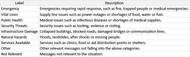
In addition, each message was permitted to have multiple labels, for example “Water Shortage” and “Medical Emergency” – which were allowed to be a mix of primary and secondary categories. These labelling complexities would make developing a model more difficult, without adding a lot of value. Instead of working with such complexities, it makes sense to use a simpler setting for model development where each message has a single label from a set of possible labels.

A simpler setting

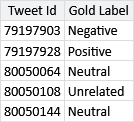
The problem of inferring high quality labels from a large number of noisy crowd-sourced annotations arises in many applications. To investigate how well different approaches work at scale a company called CrowdFlower (now Appen) ran the CrowdScale Shared Task Challenge, back in 2013. In this competition, different systems competed to see who could infer the best labels for a set of messages given a large number of noisy annotations. For the purposes of the competition, CrowdFlower created a data set of tweets about the weather, along with around 550K annotations from different crowd workers (which was an unprecedented number at the time). To assess the quality of the inferred labels, CrowdFlower also provided a high quality set of labels to be used as ground truth. In the context of crowd sourcing, such labels are often called gold labels to distinguish them from labels provided by the workers.

Figure 7.2In the CrowdFlower competition, crowd workers annotated tweets as being positive about the weather, negative about the weather, neutral about the weather or unrelated to the weather. Note the similarity between this setting and that of Figure 7.1.

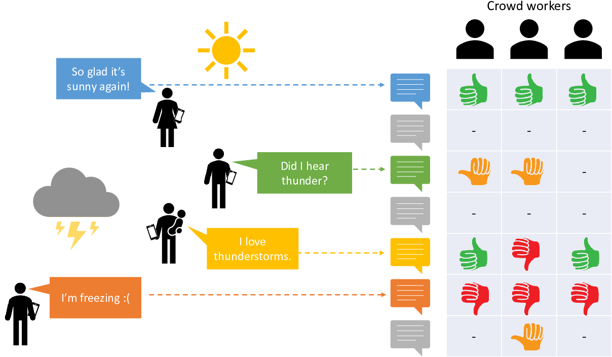
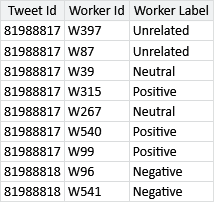
Figure 7.2 shows the setting that CrowdFlower created for their competition. Crowd workers were presented with tweets selected so as to be mostly about the weather. The task given to each crowd worker was to read a tweet and annotate with one of the labels from Table 7.2. Crowd workers were also given the option to say “Cannot tell” – rather than treat this as a label, we will take it to mean that the worker could not provide a meaningful label and so we will discard such labels. This kind of task, where the aim is to infer an author’s feelings from a piece of text is called sentiment analysis [Liu, 2012].

Excel

CSV

Table 7.2The categories which could be used to label a tweet in the CrowdFlower data set. This is a much simpler set of labels than those of Table 7.1.

The full CrowdFlower data set consists of:

• 98,920 tweets, selected so that a high proportion are about the weather;
• 540,021 labels provided by 1,958 crowd workers;
• 975 gold labels provided by expert labellers.

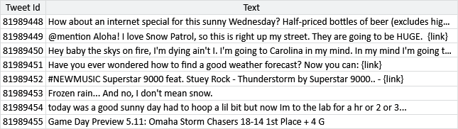
A small sample of the data set is shown in Table 7.3.

Excel

CSV

(a)Example tweets

 

Excel

CSV

(b)Example crowd worker labels

  

Excel

CSV

(c)Example gold labels

Table 7.3Sample data from the CrowdFlower data set, consisting of (a) tweets selected to be likely to be about the weather (b) worker labels and (c) gold labels.

Using more than two labels

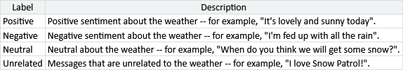
In this weather setting, the true label for each tweet can have one of four possible values: Positive, Negative, Neutral or Unrelated. We will need to have a variable in our model for this true label, which we’ll call trueLabel. As usual, we will keep track of all the assumptions we are making in building this model. So our first assumption is:

1. Each tweet has a true label which is one of the following set: Positive, Negative, Neutral or Unrelated.

Because trueLabel can take more than two values, we need to use a discrete distribution as a prior or posterior distribution for this variable. Recall that we first encountered discrete distributions back in section 6.5 when working with a sensitization class variable that could also take on more than two values. The important thing to remember is that the discrete distribution is an extension of the Bernoulli distribution for variables with more than two possible values.

When working out which label a tweet has, it is very useful to know whether some labels are more common than others. For example, if the set of tweets has been selected to be as relevant as possible, we might expect the Unrelated label to be less common. We can incorporate this knowledge into our model by learning the probability of a tweet taking on each of the labels – effectively this means learning the parameters of a discrete distribution. We have encountered a similar situation before in section 2.6, where we used a beta distribution to learn the probability of true for a Bernoulli distribution. Here, we want to learn the probabilities associated with each possible value in a discrete distribution. We need an extended form of a beta distribution, that can handle learning a set of probability values that add up to 1. Happily, such a distribution exists: it is called the Dirichlet distribution – and has a probability density function given by:

where $K$ is the number of values that the variable can have, $\mathbf{x}$ is an array of $K$ probability values adding up to 1 and $\mathbf{\alpha}$ is the array of $K$ counts that are the parameters of the distribution. Here, $\mathrm{B}()$ is the multi-variate form of the beta function that we encountered in the density of the beta distribution (section 2.6). When $K$ is 2, equation (7.1) becomes identical to the beta density given back in equation (2.22) – this means that the beta distribution is exactly the same as a Dirichlet distribution with $K=2$.

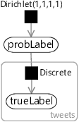
For our setting, we have four possible labels and so $K$ is equal to 4. We want to learn an array of four probabilities for each of the four possible labels. Since we want to learn this array, we need to create a random variable for it – which we shall call probLabel. Note that the value of this variable is an array of probability values, rather than just one value. We need to choose a prior distribution for probLabel to encode our knowledge about this array of probabilities before we have seen any data. Since we don’t want to assume anything about the probabilities ahead of time, we can choose a uniform Dirichlet distribution that gives equal probability to any array of probability values that sum to 1. Such a uniform Dirichlet can be created by setting all the count parameters $\mathbf{\alpha}$ to 1, which can be written as Dirichlet(1,1,1,1).

We’ve now defined two variables for our model: a trueLabel variable for each tweet and a single, global probLabel variable giving the probabilities for each label. We can connect these variables in a factor graph as shown in Figure 7.3, where the Discrete factor defines a discrete distribution over trueLabel whose parameters are the probability array probLabel. Because there is a label for each tweet, the trueLabel variable sits inside a plate across the tweets.

plate of size: tweets tweets double[] variable An array of probabilities of a tweet having each possible label. probLabel int[] variable The true label for this tweet. trueLabelDirichlet(1,1,1,1)Discrete

Figure 7.3A model where the probability of the true label for a tweet taking each possible value is given by the array of probabilities probLabel.

In the model of Figure 7.3, neither of the two variables are observed. In particular, we do not observe the trueLabel because we need to infer this from the workers’ labels. We need to extend our model then to include the crowd workers and their labels.

Incorporating crowd worker labels

We can use pieces of models from previous chapters as building blocks for our new model.

In this chapter, we will find ourselves re-using pieces of models that we have developed in previous chapters. The ability to draw on existing model components is a very useful advantage of model-based machine learning. It means that we can often construct our models out of large pre-existing pieces rather than having to design them from scratch each time.

We need to model the situation where a crowd worker is trying to work out the correct label for a tweet. This is similar to the situation in Chapter 2 where a candidate was trying to work out the correct answer for a question. In that model, we assumed that either the candidate had the skills to answer a question or not. Here, we will make a similar assumption:

2. When a worker looks at a tweet, they will either be able to work out what the true label is or not.

To model this assumption, we will use a variable for whether the worker can work out the true label or not. We’ll call this isCorrect and it will be true if the worker can work out the correct label or false otherwise.

Next we need to decide what the worker does to choose a label for the tweet. Let’s call this label workerLabel and allow it to take any of the four label values, just like trueLabel. Building on our previous assumption, if the worker can work out the true label, then we may reasonably assume that this is the label that they will provide.

3. If a worker can determine the true label, they will give this as their label.

If they cannot work out the true label, then they still need to provide some label – so we need to decide what they do in this case. In Chapter 2, we assumed that if someone did not know the answer to a question then they would just guess at random. We can make the same assumption here:

4. If a worker cannot determine the true label, they will choose a label uniformly at random.

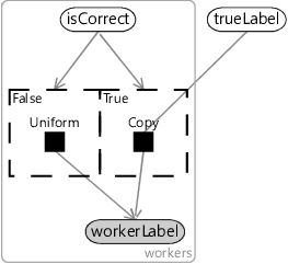
According to Assumptions0 7.3, if isCorrect is true, then workerLabel will simply be a copy of trueLabel. But according to Assumptions0 7.4, if isCorrect is false, then workerLabel must instead have a uniform distribution. To switch between these two difference ways of modelling workerLabel, we can use gates just like we did in the previous chapter (section 6.4). For Assumptions0 7.3, we need a gate which is on when isCorrect is true and which contains a Copy factor that copies the value of trueLabel into workerLabel. The Copy factor is a deterministic factor which gives probability 1.0 to the child variable having the same value as the parent variable and probability 0.0 to all other values. To model Assumptions0 7.4, we need a second gate which is on when isCorrect is false and contains a Uniform factor that gives a uniform discrete distribution to workerLabel. The resulting factor graph for a single tweet is shown in Figure 7.4.

plate of size: workers workers gate (on when isCorrect=True) True gate (on when isCorrect=False) False observed int[] variable The label assigned to this tweet by this worker. workerLabel int variable The true label for this tweet. trueLabel bool variable Whether the worker correctly worked out the true label for this tweet. isCorrect Copy Uniform

Figure 7.4Model of all the worker labels for a single tweet. Each worker can either correctly work out the true label or not, as indicated by isCorrect. If they can work out the true label then they copy it into their label (right hand gate), otherwise they pick a label uniformly at random (left hand gate). The resulting label is stored in workerLabel – this is shown shaded because the values of these labels are known to the system.

Completing the model

The model of Figure 7.4 does not provide a prior for the isCorrect variable. We could just pick one and assume, say, that worker are correct $90\%$ of the time. Instead, we will be a bit more sophisticated and allow the model to learn the probability of each worker being correct. We will call this the ability of the worker and put it inside a plate over the workers to give each worker there own ability. The assumption we will make is:

5. Some workers will be able to determine the true label more often than others, but most will manage most of the time.

Since we expect most workers to determine the true label most of the time, we will give ability a prior distribution that favours probabilities above $50\%$. A Beta(2,1) distribution is a reasonable choice here.

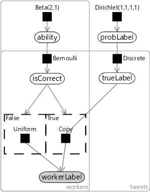
We can now put together factor graphs Figure 7.3 and Figure 7.4, along with this new ability variable to give the overall factor graph of Figure 7.5. Here we have placed the single tweet model of Figure 7.4 inside a plate over tweets, added in probLabel from Figure 7.4 and added the ability variable as a parent to isCorrect.

plate of size: tweets tweets plate of size: workers workers gate (on when isCorrect=True) True gate (on when isCorrect=False) False observed int[][] variable The label assigned to this tweet by this worker. workerLabel double[] variable An array of probabilities of a tweet having each possible label. probLabel int[] variable The true label for this tweet. trueLabel double[] variable The ability of a worker is the probability that they can work out the true label for a tweet. ability bool variable Whether the worker correctly worked out the true label for this tweet. isCorrectDirichlet(1,1,1,1)DiscreteBeta(2,1)Bernoulli Copy Uniform

Figure 7.5The overall model of a set of crowd workers labelling a set of tweets. Each worker has a different ability indicating the proportion of tweets that they will label correctly.

As usual, we should now take a moment to review our modelling assumptions. They are shown all together in Table 7.4.

Assumptions0 7.1 is given by the setting, so is a safe assumption. Assumptions0 7.2 also seems safe since surely the worker can either work out the correct label or not. Assumptions0 7.3 is a reasonable assumption if we believe that workers are genuinely trying to be helpful and not deliberately providing incorrect values. If we instead believe that there are workers trying to undermine the correct labelling, then we would need to revisit this assumption. Assumptions0 7.4 is a simplifying assumption – in practice, workers will rarely pick at random but might instead make a best guess – this assumption may well be worth refining later. Finally, Assumptions0 7.5 seems like a reasonable assumption as long as we believe that the labelling task is easy enough for most workers most of the time. If this is not true, then we are probably in trouble anyway!

We now have a complete model and are ready to try it out – read on to see how well it works.