1.1 Incorporating evidence

Dr Bayes searches the mansion thoroughly. She finds that the only weapons available are an ornate ceremonial dagger and an old army revolver. “One of these must be the murder weapon”, she concludes.

So far, we have considered just one random variable: murderer. But now that we have some new information about the possible murder weapons, we can introduce a new random variable, weapon, to represent the choice of murder weapon. This new variable can take two values: revolver or dagger. Given this new variable, the next step is to use probabilities to express its relationship to our existing murderer variable. This will allow us to reason about how these variables affect each other and to make progress in solving the murder.

Suppose Major Grey were the murderer. We might believe that the probability of his choosing a revolver rather than a dagger for the murder is, say, 90% on the basis that he would be familiar with the use of such a gun from his time in the army. But if instead Miss Auburn were the murderer, we might think the probability of her using a revolver would be much smaller, say 20%, since she might be unfamiliar with the operation of a weapon which went out of use before she was born. This means that the probability distribution over the random variable weapon depends on whether the murderer is Major Grey or Miss Auburn. This is known as a conditional probability distribution because the probability values it gives vary depending on another random variable, in this case murderer. If Major Grey were the murderer, the conditional probability of choosing the revolver can be expressed like so:

Here the quantity on the left side of this equation is read as “the probability that the weapon is the revolver given that the murderer is Grey”. It describes a probability distribution over the quantity on the left side of the vertical ‘conditioning’ bar (in this case the value of weapon) which depends on the value of any quantities on the right hand side of the bar (in this case the value of murderer). We also say that the distribution over weapon is conditioned on the value of murderer.

Since the only other possibility for the weapon is a dagger, the probability that Major Grey would choose the dagger must be 10%, and hence

Again, we can also express this information in pictorial form, as shown in Figure 1.3.

Figure 1.3Representation of the probabilities for the two weapons, conditional on Major Grey being the murderer.

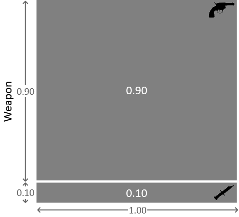
Here we see a square with a total area of 1.0. The upper region, with area 0.9, corresponds to the conditional probability of the weapon being the revolver, while the lower region, with area 0.1, corresponds to the conditional probability of the weapon being the dagger. If we pick a point at random uniformly from within the square (in other words, sample from the distribution), there is a 90% probability that the weapon will be the revolver.

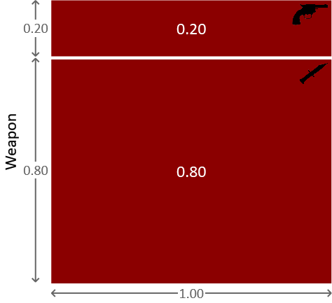
Now suppose instead that it was Miss Auburn who committed the murder. Recall that we considered the probability of her choosing the revolver was 20%. We can therefore write

Again, the only other choice of weapon is the dagger and so

This conditional probability distribution can be represented pictorially as shown in Figure 1.4.

Figure 1.4Representation of the probabilities for the two weapons, conditional on Miss Auburn being the murderer.

We can combine all of the above information into the more compact form

This can be expressed in an even more compact form as $P(\var{weapon} | \var{murderer})$. As before, we have a normalization constraint which is a consequence of the fact that, for each of the suspects, the weapon used must have been either the revolver or the dagger. This constraint can be written as

where the sum is over the two states of the random variable weapon, that is for weapon=revolver and for weapon=dagger, with murderer held at any fixed value (Grey or Auburn). Notice that we do not expect that the probabilities add up to 1 over the two states of the random variable murderer, which is why the two numbers in equation (1.10) do not add up to 1. These probabilities do not need to add up to 1, because they refer to the probability that the revolver was the murder weapon in two different circumstances: if Grey was the murderer and if Auburn was the murderer. For example, the probability of choosing the revolver could be high in both circumstances or low in both circumstances – so the normalization constraint does not apply.

Conditional probabilities can be written in the form of a conditional probability table (CPT) – which is the form we will often use in this book. For example, the conditional probability table for $P(\var{weapon} | \var{murderer})$ looks like this:

Table 1.1The conditional probability table for $P(\var{weapon} | \var{murderer})$. Table columns correspond to values of the conditioned variable weapon, rows correspond to values of the conditioning variable murderer, and table cells contain the conditional probability values. The normalization constraint means that the values in any row must add up to 1. We have also added blue bars to the table to provide a visual indication of the probability values.

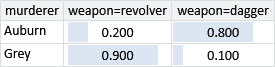
As we just discussed, the normalization constraint means that the probabilities in the rows of Table 1.1 must add up to 1, but not the probabilities in the columns.

Independent variables

We have assumed that the probability of each choice of weapon changes depending on the value of murderer. We say that these two variables are dependent. More commonly, we tend to focus on what variables do not affect each other, in which case we say they are independent variables. Consider for example, whether it is raining or not outside the Old Tudor Mansion at the time of the murder. It is reasonable to assume that this variable raining has no effect whatsoever on who the murderer is (nor is itself affected by who the murderer is). So we have assumed that the variables murderer and raining are independent. You can test this kind of assumption by asking the question “Does learning about the one variable, tell me anything about the other variable?”. So in this case, the question is “Does learning whether it was raining or not, tell me anything about the identity of the murderer?”, for which a reasonable answer is “No”.

If we tried to write down a conditional probability for $P(\var{raining}|\var{murderer})$, then it would give the same probability for raining whether murderer was Grey or Auburn. If this were not true, learning about one variable would tell us something about the other variable, through a change in its probability distribution. We can express independence between these two variables mathematically.

What this equation says is that the probability of raining given knowledge of the murderer is exactly the same as the probability of raining without taking into account murderer. In other words, the two variables are independent. This also holds the other way around:

Independence is an important concept in model-based machine learning, since any variable we do not explicitly include in our model is assumed to be independent of all variables in the model. We will see further examples of independence later in this chapter.

Let us take a moment to recap what we have achieved so far. In the first section, we specified the probability that the murderer was Major Grey (and therefore the complementary probability that the murderer was Miss Auburn). In this section, we also wrote down the probabilities for different choices of weapon for each of our suspects. In the next section, we will see how we can use all these probabilities to incorporate evidence from the crime scene and reason about the identity of the murderer.