4.3 Modelling multiple features

With just one feature, our classification model is not very accurate at predicting reply, so we will now extend it to handle multiple features. We can do this by changing the model so that multiple features contribute to the score for an email. We just need to decide how to do this, which involves making an additional assumption:

6. A particular change in one feature’s value will cause the same change in score, no matter what the values of the other features are.

Let’s consider this assumption applied to the ToLine feature and consider changing it from 0.0 to 1.0. This assumption says that the change in score due to this change in feature value is always the same, no matter what the other feature values are. This assumption can be encoded in the model by ensuring that the contribution of the ToLine feature to the score is always added on to the contributions from all the other features. Since the same argument holds for each of the other features as well, this assumption means that the score for an email must be the sum of the score contributions from each of the individual features.

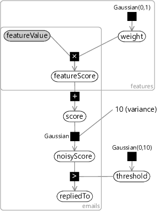
So, in our multi-feature model (Figure 4.5), we have a featureScore array to hold the score contribution for each feature for each email. We can then use a deterministic summation factor to add the contributions together to give the total score. Since we still want Assumptions0 4.3 to hold for each feature, the featureScore for a feature can be defined, as before, as the product of the featureValue and the feature weight. Notice that we have added a new plate across the features, which contains the weight for the feature, the feature value and the feature score. The value and the score are also in the emails plate, since they vary from email to email, whilst the weight is outside since it is shared among all emails.

plate of size: features features plate of size: emails emails observed double[][] variable The value of this feature. featureValue double[] variable The weight for this feature. weight double variable The threshold score for replying. threshold double[][] variable The score for this feature, which is the product of the feature value and the feature weight. featureScore double[] variable The total score for this email. score double[] variable Score with added Gaussian noise. noisyScore double variable 10 (variance) bool[] variable Whether the message is replied to. repliedToGaussian(0,1)Gaussian(0,10)×+Gaussian>

Figure 4.5Factor graph of a classification model with multiple features. Variables within the features plate are duplicated for each feature, so there is a separate weight for each feature and, for each email, a separate featureValue and featureScore. The featureScore values for each feature are summed to give an overall score for each email.

We now have a model which can combine together an entire set of features. This means we are free to put in as many features as we like, to try to predict as accurately as possible whether a user will reply to an email. More than that, we are assuming that anything we do not put in as a feature is not relevant to the prediction. This is our final assumption:

7. Whether the user will reply to an email depends only on the values of the features and not on anything else.

As before, now that we have a complete model, it is a good exercise to go back and review all the assumptions that we have made whilst building the model. The full set of assumptions is shown in Table 4.3.

Assumptions0 4.1 arises because we chose to build a conditional model, and so we need to always condition on the feature values.

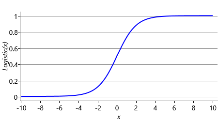
In our model, we have used the red curve of Figure 4.3 to satisfy Assumptions0 4.2. Viewed as a function that computes the score given the reply probability, this curve is called the probit function. It is named this way because the units of the score have historically been called ‘probability units’ or ‘probits’ [Bliss, 1934]. Since regression is the term for predicting a continuous value (in this case, the score) from some feature values, the model as a whole is known as a probit regression model (or in its fully probabilistic form as the Bayes Point Machine [Herbrich et al., 2001]). There are other functions that we could have used to satisfy Assumptions0 4.2 – the most well-known is the logistic function, which equals $1/(1+e^{-x})$ and has a very similar S-shape (see Figure 4.6 to see just how similar!). If we had used the logistic function instead of the probit function, we would have made a logistic regression model – a very widely used classifier. In practice, both models are extremely similar – we used a probit model because it allowed us to build on the factors and ideas that you learned about in the previous chapter.

Excel

CSV

Figure 4.6The logistic function scaled horizontally to match the Gaussian CDF from Figure 4.3. The similarity of the two functions means that our probit regression model behaves very similarly to a logistic regression model.

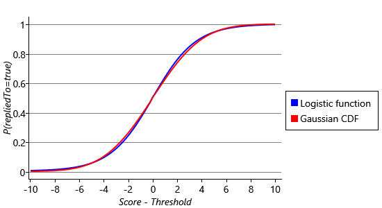
Assumptions0 4.3, taken together with Assumptions0 4.6, means that the score must be a linear function of the feature values. For example, if we had two features, the score would be $\var{weight}_1 \times \var{featureValue}_1 + \var{weight}_2 \times \var{featureValue}_2$. We use the term linear, because if we plot the first feature value against the second, then points with the same score will form a straight line. Any classifier based around a linear function is called a linear classifier.

Assumptions0 4.4 and Assumptions0 4.5 are reasonable statements about how features affect the predicted probability. However, Assumptions0 4.6 places some subtle but important limitations on what the classifier can learn, which are worth understanding. These are explored and explained in Panel 4.2.

Panel 4.2How features combine together

Assumptions0 4.6 is quite a strong assumption about how features combine together. To investigate the effect of this assumption, consider a two-feature model with the existing ToLine feature and a new feature called FromManager. This new FromManager feature has a value of 1.0 if the sender is the user’s manager and 0.0 otherwise. Suppose a particular user replies to 80% of emails from their manager, but only if they are on the To line. If they are not on the To line, then they treat it like any other email where they are on the Cc line. To analyse such a user, we will create a synthetic data set to represent our hypothetical user’s email data. For email where FromManager is zero, we will take User35CB8E5’s data set from Table 4.2b. We will then add 500 new synthetic emails where FromManager is 1, such that the user is on the To line exactly half of the time, giving the data set in the table below. The final column of this table gives the predicted probabilities for each combination of features, for a model trained on this data.

Excel

CSV

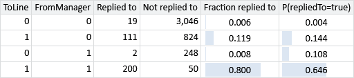
There is quite a big difference between the predicted probability of reply and the actual fraction replied to. For example, the predicted probability for emails from the user’s manager where the user is on the To line is much too low: 64.6% not 80%. Similarly, the prediction is too high (10.8% not 0.8%) for emails from the user’s manager where the user is not on the To line. These inaccurate predictions occur because there is no setting of the weight and threshold variables that can make the predicted probability match the actual reply fraction. Assumptions0 4.6 says the change in score for FromManager must be the same when ToLine is 1.0 as for when ToLine is 0.0. But, to match the data, we need the change in score to be higher when ToLine is 1.0 than when it is 0.0.

Rather than changing the model to remove Assumptions0 4.6, we can work around this limitation by adding a new feature that is 1.0 only if ToLine and FromManager are both 1.0 (an AND of the two features). This new feature will have its own weight associated with it, which means there can now be a different score for manager emails when the user is on the To line to when they are not on the To line. If we train such a three-feature model, we get the new predictions shown here:

Excel

CSV

The predicted probabilities are now much closer to the actual reply fractions in each case, meaning that the new model is making more accurate predictions than the old one. Any remaining discrepancies are due to Assumptions0 4.5, which controls the size of effect of any single feature.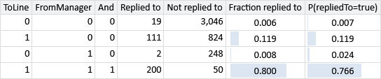

This problem can be avoided by always using an AND of the values of a subset of features. This is the approach taken in a decision tree model, a non-linear classifier which we will discuss in section 8.2. When training a decision tree, we are effectively searching for combinations of features like the one above, which lead to good predictions. Unfortunately, decision trees suffer from a different problem, where the values of many features are ignored when making a prediction. A popular solution to both issues is to combine several decision trees together through a linear model into a decision forest – this approach is also discussed in section 8.2.

Finally, Assumptions0 4.7 states that our feature set contains all of the information that is relevant to predicting whether a user will reply to an email. We’ll see how to develop a feature set to satisfy this assumption as closely as possible in the next section, but first we need to understand better the role that the feature set plays.

Features are part of the model

To use our classification model, we will need to choose a set of features to transform the data, so that it better conforms to the model assumptions of Table 4.3. Another way of looking at this is that the assumptions of the combined feature set and classification model must hold in the data. From a model-based machine learning perspective, this means that the feature set combined with the classification model form a larger overall model. In this way of looking at things, the feature set is the part of this overall model that is usually easy to change (by changing the feature calculation code) whereas the classification part is the part that is usually hard to change (for example, if you are using off-the-shelf classifier software there is no easy way to change it).

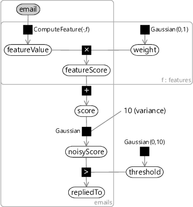
We can represent this overall combined model in a factor graph by including the feature calculations in the graph, as shown in Figure 4.7. The email variable holds all the data about the email itself (you can think of it as an email object). The feature calculations appear as deterministic ComputeFeature factors inside of the features plate, each of which computes the feature value for the feature, given the email. Notice that, although only email is shown as observed (shaded), featureValue is effectively observed as well since it is deterministically computed from email.

plate of size: features f : features plate of size: emails emails observed Email[] variable email double[][] variable The value of this feature. featureValue double[] variable The weight for this feature. weight double variable The threshold score for replying. threshold double[][] variable The score for this feature, which is the product of the feature value and the feature weight. featureScore double[] variable The total score for this email. score double[] variable Score with added Gaussian noise. noisyScore double variable 10 (variance) bool[] variable Whether the message is replied to. repliedToGaussian(0,1)Gaussian(0,10)ComputeFeature(·,f)×+Gaussian>

Figure 4.7Factor graph of a model which includes both feature calculation and classification. The ComputeFeature factor takes as arguments the current feature $f$ and the email being considered and computes the value of feature $f$ for that email.

If the feature set really is part of the model, we must use the same approach for designing a feature set, as for designing a model. This means that we need to visualise and understand the data, be conscious of assumptions being represented, specify evaluation metrics and success criteria, and repeatedly refine and improve the feature set until the success criteria are met (in other words, we need to follow the machine learning life cycle). This is exactly the process we will follow next.

logistic functionThe function $f(x) = 1/(1+e^{-x})$ which is often used to transform unbounded continuous values into continuous values between 0 and 1. It has an S-shape similar to that of the cumulative Gaussian (see Figure 4.6).

Excel

CSV