A Murder Mystery

As the clock strikes midnight in the Old Tudor Mansion, a raging storm rattles the shutters and fills the house with the sound of thunder. The dead body of Mr Black lies slumped on the floor of the library, blood still oozing from the fatal wound. Quick to arrive on the scene is the famous sleuth Dr Bayes, who observes that there were only two other people in the Mansion at the time of the murder. So who committed this dastardly crime? Was it the fine upstanding pillar of the establishment Major Grey? Or was it the mysterious and alluring femme fatale Miss Auburn?

We begin our study of model-based machine learning by investigating a murder. Although seemingly simple, this murder mystery will introduce many of the key concepts that we will use throughout the book. You can reproduce all results in this chapter for yourself using the companion source code [Diethe et al., 2019].

The goal in tackling this mystery is to work out the identity of the murderer. Having only just discovered the body, we are very uncertain as to whether the murder was committed by Miss Auburn or Major Grey. Over the course of investigating the murder, we will use clues discovered at the crime scene to reduce this uncertainty as to who committed the murder.

Immediately we face our first challenge, which is that we have to be able to handle quantities whose values are uncertain. In fact the need to deal with uncertainty arises throughout our increasingly data-driven world. In most applications, we will start off in a state of considerable uncertainty and, as we get more data, become increasingly confident. In a murder mystery, we start off very uncertain who the murderer is and then slowly get more and more certain as we uncover more clues. Later in the book, we will see many more examples where we need to represent uncertainty: when two players play each other in Xbox live it is more likely that the stronger player will win, but this is not guaranteed; we can be fairly sure that a user will reply to a particular email but we can never be certain.

Consequently, we need a principled framework for quantifying uncertainty which will allow us to create applications and build solutions in ways that can represent and process uncertain values. Fortunately, there is a simple framework for manipulating uncertain quantities which uses probability to quantify the degree of uncertainty. Many people are familiar with the idea of probability as the frequency with which a particular event occurs. For example, we might say that the probability of a coin landing heads is 50% which means that in a long run of flips, the coin will land heads approximately 50% of the time. In this book we will be using probabilities in a much more general sense to quantify uncertainty, even for situations, such as a murder, which occur only once.

(a)Major Grey

  

(b)Miss Auburn

Figure 1.1Is the murderer Major Grey or Miss Auburn? Probabilities allow us to express how certain we are that a particular suspect is the murderer.

Let us apply the concept of probability to our murder mystery. The probability that Miss Auburn is the murderer can range from 0% to 100%, where 0% means we are certain that Miss Auburn is innocent, while 100% means we are certain that she committed the murder. We can equivalently express probabilities on a scale from 0 to 1, where 1 is equivalent to 100%. From what we know about our two characters, we might think it is unlikely that someone with the impeccable credentials of Major Grey could commit such a heinous crime, and therefore our suspicion is directed towards the enigmatic Miss Auburn. Therefore, we might assume that the probability that Miss Auburn committed the crime is 70%, or equivalently 0.7.

To express this assumption, we need to be precise about what this 70% probability is referring to. We can do this by representing the identity of the murderer with a random variable – this is a variable (a named quantity) whose value we are uncertain about. We can define a random variable called murderer which can take one of two values: it equals either Auburn or Grey. Given this definition of murderer, we can write our 70% assumption in the form

where the notation $P(\ )$ denotes the probability of the quantity contained inside the brackets. Thus equation (1.1) can be read as “the probability that the murderer was Miss Auburn is 70%”. Our assumption of 70% for the probability that Auburn committed the murder may seem rather arbitrary – we will work with it for now, but in the next chapter we shall see how such probabilities can be learned from data.

We know that there are only two potential culprits and we are also assuming that only one of these two suspects actually committed the murder (in other words, they did not act together). Based on this assumption, the probability that Major Grey committed the crime must be 30%. This is because the two probabilities must add up to 100%, since one of the two suspects must be the murderer. We can write this probability in the same form as above:

We can also express the fact that the two probabilities add up to 1.0:

This is an example of the normalization constraint for probabilities, which states that the probabilities of all possible values of a random variable must add up to 1.

If we write down the probabilities for all possible values of our random variable murderer, we get:

Written together this is an example of a probability distribution, because it specifies the probability for every possible state of the random variable murderer. We use the notation $P(\var{murderer})$ to denote the distribution over the random variable murderer. This can be viewed as a shorthand notation for the combination of $P(\var{murderer} = \state{Auburn})$ and $P(\var{murderer} = \state{Grey})$. As an example of using this notation, we can write the general form of the normalization constraint:

where the symbol ‘$\sum$’ means ‘sum’ and the subscript ‘murderer’ indicates that the sum is over the states of the random variable murderer, i.e. Auburn and Grey. Using this notation, the states of a random variable do not need to be listed out – very useful if there are a lot of possible states!

At this point it is helpful to introduce a pictorial representation of a probability distribution that we can use to explain some of the later calculations. Figure 1.2 shows a square of area 1.0 which has been divided in proportion to the probabilities of our two suspects being the murderer.

Figure 1.2Representation of probabilities using areas. The grey area represents the probability that Major Grey is the murderer and the red area represents the probability that Miss Auburn is the murderer.

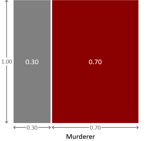
The square has a total area of 1.0 because of the normalization constraint, and is divided into two regions. The region on the left has an area of 0.3, corresponding to the probability that Major Grey is the murderer, while the region on the right has an area of 0.7, corresponding to the probability that Miss Auburn is the murderer. The diagram therefore provides a simple visualization of these probabilities. If we pick a point at random within the square, then the probability that it will land in the region corresponding to Major Grey is 0.3 (or equivalently 30%) and the probability that it will land in the region corresponding to Miss Auburn is 0.7 (or equivalently 70%). This process of picking a value for a random variable, such that the probability of picking a particular value is given by a certain distribution is known as sampling. Sampling can be very useful for understanding a probability distribution or for generating synthetic data sets – later in this book we will see examples of both of these.

The Bernoulli distribution

The technical term for this type of distribution over a two-state random variable is a Bernoulli distribution, which is usually defined over the two states true and false. For our murder mystery, we can use true to mean Auburn and false to mean Grey. Using these states, a Bernoulli distribution over the variable murderer with a 0.7 probability of true (Auburn) and a 0.3 probability of false (Grey) is written $\dist{Bernoulli}(\var{murderer};0.7)$. More generally, if the probability of murderer being true is some number $p$, we can write the distribution of murderer as $\dist{Bernoulli}(\var{murderer};p)$.

Often when we are using probability distributions it will be unambiguous which variable the distribution applies to. In such situations we can simplify the notation and instead of writing $\dist{Bernoulli}(\var{murderer};p)$ we just write $\dist{Bernoulli}(p)$. It is important to appreciate that is just a shorthand notation and does not represent a distribution over $p$. Since we will be referring to distributions frequently throughout this book, it is very useful to have this kind of shorthand, to keep notation clear and concise.

We can use the Bernoulli distribution with different values of the probability to represent different judgements or assessments of uncertainty, ranging from complete ignorance through to total certainty. For example, if we had absolutely no idea which of our suspects was guilty, we could assign $P(\var{murderer}) = \dist{Bernoulli}(\var{murderer};0.5)$ or equivalently $P(\var{murderer}) = \dist{Bernoulli}(0.5)$. In this case both states have probability 50%. This is an example of a uniform distribution in which all states are equally probable. At the other extreme, if we were absolutely certain that Auburn was the murderer, then we would set $P(\var{murderer}) = \dist{Bernoulli}(1)$, or if we were certain that Grey was the murderer then we would have $P(\var{murderer}) = \dist{Bernoulli}(0)$. These are examples of a point mass, which is a distribution where all of the probability is assigned to one value of the random variable. In other words, we are certain about the value of the random variable.

So, using this new terminology, we have chosen the probability distribution over murderer to be Bernoulli(0.7). Next, we will show how to relate different random variables together to start solving the murder.