5.3 Training our recommender

Before we can train our model, we need some data to train it on. The good news here is that there are some high quality public data sets which can be used for training recommender models. We will use one of the excellent MovieLens data sets by GroupLens Research at the University of Minnesota [Harper and Konstan, 2015]. We will use a data set that has been made freely available for education and development purposes – thank you, MovieLens! You can download the data set yourself using this link.

Getting to know our data

As with any new data set, our first task is to get to know the data. First of all, here is a sample of 10 ratings from the data set:

Excel

CSV

Table 5.3A sample of ratings from the MovieLens data set.

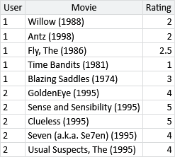
The sample shows that each rating gives the ID of the person providing the rating, the movie being rated, and the number of stars that the person gave the movie. In addition to ratings, the data set also contains some information about each movie – we’ll look at this later on, in section 5.6.

It’s a good idea to view a new data set in many different ways, to get a deeper understanding of the data and to identify any possible data issues as early as possible. As an example, let’s make a plot to understand what kind of ratings people are giving. The above sample suggests that ratings go up to 5 stars and that half stars are allowed. To confirm this and to understand how frequently each rating is given, we can plot a histogram of all the ratings in the data set.

Excel

CSV

Figure 5.12The number of ratings given for each possible number of stars (from half a star up to five stars).

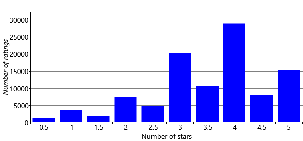
We can learn a few things about the ratings from Figure 5.12. The first is that whole star ratings are given more than nearby ratings with half stars. Secondly, the plot is biased to the right, showing that people are much more likely to give a rating above three stars than below. This could perhaps be because people are generous to the movies and try to give them decent ratings. Another possibility is that people only rate movies that they watch and they only watch movies that they expect to like. For example, someone might hate horrors movies and so would never watch them, and so never rate them. If they were forced to watch the movie, they would likely give it a very low rating. Since people are not usually forced to watch movies, such ratings would not appear in the data set, leading to the kind of rightward bias seen in Figure 5.12.

This issue of missing data is an important one and we will discuss it in detail in section 6.2 of the next chapter. For now we will just have to bear in mind that this missing data will likely have a negative effect on our prediction accuracy – since we have less data about the movies a person does not like.

Training on MovieLens data

The model we have developed allows for two possible ratings: ‘like’ or ‘dislike’. If we want to use the MovieLens data set with this model, we need a way to convert each star rating into a like or a dislike (we’ll look at how we can use the star ratings directly later). Guided by Figure 5.12, we will assume that 3 or more stars means that a person liked the movie, and that 2.5 or fewer stars means they did not like the movie. Applying the transformation gives us a data set of like/dislike ratings.

We need to split this like/dislike data into a training set for training our model, and a validation set to evaluate recommendations coming from the model. For each person we will use 70% of their likes/dislikes to train on and leave 30% to use for validation. We also remove ratings from the validation set for any movies that do not appear anywhere in the training set (since the trait position for these movies cannot be learned). The result of this process is:

• a training set of 69,983 ratings (57,383 likes/12,600 dislikes) covering 8,032 movies,
• a validation set of 28,831 ratings (23,952 likes/4,879 dislikes) covering 4,761 movies.

Both data sets contain ratings from 671 different people.

To train the model, we attach the training set data to the likesMovie variable and once again use expectation propagation to infer the trait values for each movie and the preference values for each person. However, when we try to do this, the posterior distributions for these variables remain broad and centered at zero. What is going on here?

Symmetries can cause inference problems.

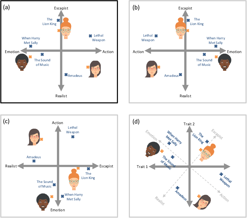
To understand the cause of this problem, let’s look again at the picture of trait space from Figure 5.9, which we’ve repeated in Figure 5.13a. The choice of having emotion on the left and action on the right was completely arbitrary. We could flip these over so that action is on the left and emotion is on the right, whilst also flipping the positions of all the people and movies correspondingly, as shown in Figure 5.13b. The result is a flipped trait space that gives exactly the same predictions. We could also swap the action/emotion trait with the escapist/realist trait, as shown in Figure 5.13c. Again the result would give exactly the same predictions. Notice that Figure 5.13c is also the same as Figure 5.13b rotated by 90-degrees to the left. We can also apply other rotations so that the axes of the plot no longer lined up with our original traits (Figure 5.13d) and we still get the same predictions! When a model’s variables can be systematically transformed without changing the resulting predictions, the model is said to contain symmetries. During inference, these symmetries cause the posterior distributions to get very broad, as they try to capture all rotations and flips of trait space simultaneously. Not helpful!

Figure 5.13Examples of symmetries in our recommender model. (a) Original trait space (b) A left-right flip symmetry (c) A flip symmetry caused by swapping the axes (d) A rotational symmetry.

To solve this inference problem, we need to do some kind of symmetry breaking. Symmetry breaking is any modification to the model or inference algorithm with the aim of removing symmetries from the posterior distributions of interest. For a two-trait version of our model, we can break symmetry by fixing the position of two points in trait space – for example, fixing the positions of the first two movies in the training set. We choose to fix the first movie to (1,0) and the second to (0,1). These two points mean that rotations and flips of the trait space now lead to different results, since these two movies cannot be rotated/flipped correspondingly – and so we have removed the symmetries from our model.

With symmetry breaking in place, EP now converges to a meaningful result. However, the EP message passing algorithm runs extremely slowly due to the high cost of computing messages relating to the product ($\times$) factor. In Stern et al. [2009] a variation of the EP message calculation is used for these messages (as shown in equation (6) in the paper), which has the effect of speeding up the message calculation dramatically.

This faster inference algorithm gives posteriors over the position in trait space for each movie and each person. In many cases, these posteriors are quite broad because there were not enough ratings to place the movie or person accurately in trait space. In Figure 5.14, we plot the inferred positions of those movies where the posterior was narrow enough to locate the movie reasonably precisely. Specifically, we plot a point at the posterior mean for each movie where the posterior variance is less than 0.2 in each dimension – this means that points are plotted for only 158 of our 8,032 movies. The learned positions of people in trait space are distributed in broadly similar fashion to the positions of movies, and so we will not show a plot of their positions.

Figure 5.14Learned positions of movies in trait space. For readability, only a subset of points have been labelled with the name of the movie (centered on the corresponding point). The two ‘anchor’ movies, The Usual Suspects and Mulholland Drive are shown in red at (0,1) and (1,0).

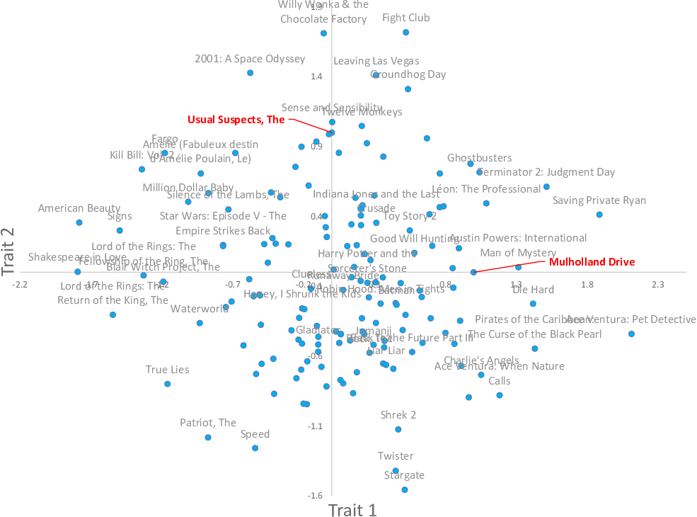
This plot shows that our model has been able to learn two traits and assign values for these traits to some movies, entirely using ratings – a pretty incredible achievement! We can see that the learned trait values have some reassuring characteristics – for example, movies in the same series have been placed near each other (such as the two Lord of the Rings movies or the two Ace Ventura movies). This alone is pretty incredible – our system had no idea that these movies were from the same series, since it was not given the names of the movies. Just using the like/dislike ratings alone, it has placed these movies close together in trait space! Beyond these characteristics, it is hard to interpret much about the traits themselves at this stage. Instead, we’ll just have to see how useful they are when it comes to making recommendations.