6.2 Trying out the model

Now that we have a complete model, we are ready to try it out on some study data. As we’ve emphasised many times before in this book, when using a real data set, it is essential to look carefully at the data set to make sure that it is complete, correct and has the form that you expect. Remember that many common machine learning problems are caused by problems with data (such as those listed in section 2.5). A good way to check your data set is to construct visualisations that let you to see at a glance what it looks like. In this case, we need to create visualisations of the test results for each child, allergen and time point. However, this study data set contains private medical data and so we cannot share the data publicly in this book, even in the form of a visualisation. The most important thing that we learned from doing this visualisation is that there are a lot of test results missing from the data set.

When there are missing data, it is always worth analysing to understand why they are missing. In Figure 6.6, we plot the number of test results in the data set (whether positive or negative) for each age and type of test.

Excel

CSV

Figure 6.6The test results recorded for each of the two types of tests, split by age of child.

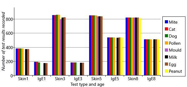
You can see several different patterns of missing data in Figure 6.6. First, the plot shows that there are ages and test types that have no data for particular allergens. For example, peanut has no results at all for ages 1 and 3, and only IgE results at age 5. Mould has no IgE results at all, and no skin test results at age 1. Second, there is a lot more missing data at early ages, particularly age 1. Third, the plot shows that there is a lot more missing data overall for IgE tests than skin tests. We need to take into consideration the effect of all these missing data points.

Working with missing data

Missing data can obscure or distort the patterns in a data set

Missing data can introduce bias into the posterior distributions computed by running inference on a model, leading to incorrect or misleading results. Whether or not this effect will occur, and how big the bias will be, depends on why the data points are missing in the first place. In statistics, it is common to consider three kinds of missingness, which are referred to using the following (quite confusing!) terms:

• missing completely at random (MCAR) – where the missing data points occur entirely at random. In other words, the fact that the data is missing is independent of the value of the missing data point (the test result that would have been given had the test actually happened).

  When data is MCAR, the remaining, non-missing, data points are effectively just a random subset of the overall data set. In this case, the posterior distributions computed by probabilistic inference will be unbiased by the missing data. Unfortunately, in reality, missing data is rarely missing completely at random. However, it may be an acceptable approximation to assume that it is – in which case, this assumption should be made with full understanding of the possibility of introducing biases.

• missing at random (MAR) – where the missingness is not random, but where other known data values fully account for the fact that the data is missing. For example, suppose that boys are more likely to refuse an IgE test than girls. Considering the fact that boys are more likely to have allergies, this would introduce a bias in our results, since the missing tests would be more likely to be positive than the non-missing tests.

  When data is MAR, it is possible to correct for the bias, at least to some extent, by changing the model appropriately to account for why the data is missing. This extension requires creating a new variable in the model for each data point, which is true if the data point is missing and false otherwise, and then building a suitable sub model to explain this new variable. For example, if boys are more likely than girls to skip an IgE test, then to correct for bias we would need to extend our model to represent this effect, such as by adding a new gender variable connected to the missingness variable. We would also need to allow this gender variable to affect the probability of sensitization in an appropriate way. The degree to which this approach corrects the bias introduced by missing data, depends on how good the model of missingness is. As ever, a better model will give better results.

• missing not at random (MNAR) – where the missingness is not either MCAR or MAR. In this case, the fact that a data point is missing depends on the value of that data point. For example, this would occur if children with lots of allergies were more likely to skip a skin prick test because of concerns about the discomfort involved in having a positive test. Or such children might be more used to medical interventions and so may be less likely to skip a blood test due to fear of needles.

  When data is MNAR, it is not possible to correct for the bias without making modelling assumptions about the nature of the bias (which could be dangerous as there would be no data to verify such assumptions). One possible approach would be to try and collect additional information relevant to why the data is missing, in the hope that this would now make it missing at random (MAR).

For more information on handling missing data, see Little and Rubin [2014].

For our study, we need to find out why the various patterns of missing data arose. Consulting again with the MAAS team, we find that:

1. The clinicians chose to omit mould tests at age 1, since this is a rare allergy and there was a desire to minimise the number of tests performed on babies. Similarly, a decision was made half way through the study to add in peanut tests.
2. The reduced number of tests at age 1 are due to manpower limitations as the study was ramped up – not all children could be brought in for testing by age 1.
3. The greater number of missing IgE tests are due to children not wanting to give blood, or parents not wanting babies or young children to have blood taken.

For 1, we know why the data is missing - because the clinicians chose not to do certain tests. Such data can be assumed to be missing completely at random, since the choice of which tests to perform at each age was made independently of any test results. For 2, the study team chose whether to invite a child in for testing by age 1 and so could choose in a way that was not influenced by the child’s allergies (such as, at random). So again, we could assume such data to be missing completely at random. For 3, we might be more concerned, as now it is a decision of the child or the parents that is influencing whether the test is performed. This is more likely to be affected by the child’s allergies, as we discussed above, and so it is possible that such missing data is not missing completely at random. For the sake of simplicity, we will assume that it is – this is such an important assumption that we should record it:

6. Missing test results are missing completely at random.

Having made this assumption, we should bear in mind that our inference results may contain biases. One reassuring point is that where we do not have an IgE test result, we often have a skin test result. This means that we still have some information about the underlying sensitization state even when an IgE test result is missing, which is likely to diminish any bias caused by its missingness.

There is another impact of missing data. Even when missing data is not introducing bias, if there is a lot of missing data it can lead to uncertainty, in the form of very broad posterior distributions. For example, at several time points we have no data for mould or peanut and so the gain/retain probabilities for those ages would be very uncertain, and so have broad posterior distributions. When included in results plots, such broad distributions can distract from the remaining meaningful results. To keep our plots as clear as possible, we will simply drop the mould and peanut allergens from our data set and consider only the remaining six allergens.

Some initial results

Having decided to treat our missing data as missing completely at random, we are now in a position to apply expectation propagation to our model and get some results. Where we have a missing data point, we simply do not observe the value of the corresponding random variable.

Having run our inference algorithm, the first posterior distributions we will look at are those for probSkinIfSens, probSkinIfNotSens, probIgeIfSens and probIgeIfNotSens. These posteriors are beta distributions, which we can summarise using a mean plus or minus a value indicating the width of the beta distribution, as shown in Table 6.3.

Excel

CSV

Table 6.3The probability of a positive test for each test type and for each sensitization state. The plus/minus values indicate the uncertainty in the probability given by the posterior beta distributions. The table shows that the skin test has a low false positive probability, but also a lower true positive probability. Conversely, the IgE test has a higher false positive probability, but a very high true positive probability. These results show that, taken together, the tests have complementary strengths and weaknesses.

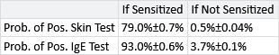
The results in Table 6.3 show that the two types of test are complementary: the skin prick test has a very low false positive rate (<1%) but as a result has a reduced true positive rate ($\sim79\%$); in contrast, the IgE test has a high true positive rate ($\sim93\%$) but as a result has a higher false positive rate ($\sim4\%$). The complementary nature of the two tests show why they are both used together – each test brings additional information about the underlying sensitization state of the child. During inference, our model will automatically take these true and false positive rates into account when inferring the sensitization state at each time point, so it will gain the advantage of the strengths of both tests, whilst being able to minimise the weaknesses.

Next let’s look at the inferred probabilities of initially having, gaining and retaining sensitization for each allergen. Figure 6.7a shows the probability of initially having a sensitization (age 1) and then the probability of gaining sensitization (ages 3, 5, 8). Similarly, Figure 6.7b shows the probability of retaining sensitization since the previous time point (for ages 3, 5 and 8 only). Since each probability has a beta posterior distribution, the charts show the uncertainty associated with the probability values, using the lower and upper quartiles of each beta distribution.

Excel

CSV

(a)The probability of having sensitivity (age 1) or subsequently gaining sensitivity (ages 3, 5 and 8).

    

Excel

CSV

(b)The probability of retaining sensitivity since the previous time point at ages 3, 5 and 8.

Figure 6.7Plots showing the probabilities for (a) having/gaining and (b) retaining sensitization for each time point and allergen.

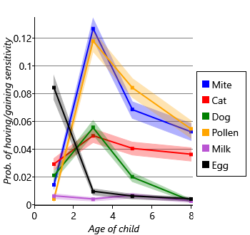
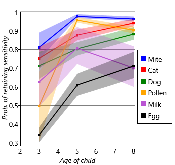
Looking at Figure 6.7a and Figure 6.7b together, we can see that different allergens have different patterns of onset and loss of sensitization. For example, there is a high initial probability of sensitivity to egg but, after that, a very low probability of gaining sensitivity. Egg also has the lowest probability of retaining sensitization, meaning that children tend to have egg sensitivity very early in life and then rapidly lose it. As another example, mite and pollen have very low initial probabilities of sensitization, but then very high probabilities of gaining sensitization by age 3. Following sensitization to mite or pollen, the probability of retaining that sensitization is very high. In other words, children who gain sensitization to mite or pollen are most likely to do so between ages 1 and 3 and will then likely retain that sensitization (at least to age 8). Cat and dog have similar patterns of gain and loss to each other, but both have a higher initial probability of sensitization and a lower peak than mite and pollen. Milk shows the lowest probabilities of sensitization, meaning that it is a rare allergy in this cohort of children. As a result, the probability of retaining a milk sensitization is more uncertain, since it is learned from relatively few children. This uncertainty is shown by the broad shaded region for milk in Figure 6.7b.

Another way of visualizaing these results, is to look at the inferred sensitizations. We have inferred the posterior probability of each child having a sensitization to each allergen at each time point. We can then count the number of children who are more likely to be sensitized than not sensitized (that is, where the probability is >50%). Plotting this count of sensitizations for each allergen and age gives Figure 6.8.

Excel

CSV

Figure 6.8The number of children with inferred sensitizations for each allergen, at each point in time.

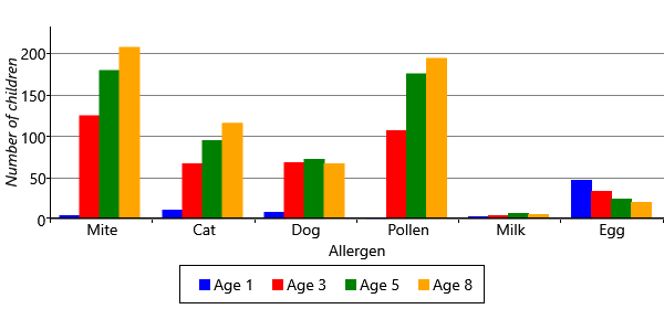
Figure 6.8 shows the patterns of gaining and losing sensitization in a different way, by showing the count of sensitized children. The chart shows that egg allergies start off common and disappear over time. The chart also shows that mite and pollen allergies start between ages 1 and 3 and the total number of allergic children only increases with age. In many ways, this chart is easier to read than the line charts of Figure 6.7a and Figure 6.7b because it looks directly at the counts of sensitizations rather than at changes in sensitizations. Also, all the information appears on one chart rather than two. For this reason, we will use this kind of chart to present results as we evolve the model later in the chapter.

To summarize, we have built a model that can learn about the patterns of gaining and losing allergic sensitization. The patterns that we have found apply to the entire cohort of children – effectively they are patterns for the population as a whole. What the model does not tell us is whether there are groups of children within the cohort that have different patterns of allergic sensitization, which might give rise to different diseases. By looking at all children together, this information is lost. Reviewing our assumptions, the problematic assumption is this one:

5. The probabilities relating to initially having, gaining or retaining sensitization to a particular allergen are the same for all children.

We’d really like to change the assumption to allow children to be in different groups, where each group of children can have different patterns of sensitization. Let’s call these groups ‘sensitization classes’. The assumption would then be:

5. The probabilities relating to initially having, gaining or retaining sensitization to a particular allergen are the same for all children in each sensitization class.

The problem is that we do not know which child is in which sensitization class. We need a model that can represent alternative processes for gaining and losing sensitization, and which can determine which process took place for each individual child. In other words, we need to be able to compare alternative models for each child’s data and determine which is likely to be the one that gave rise to the data. To achieve this will require some new tools for modelling and inference, which we will introduce in the next section.