-

Want a paper copy?
You can now buy the book!
All royalties go to the Cystic Fibrosis Trust.Spotted an error? Have comments?
Let us know!Get hands on with source code for the book.
6.3 Comparing alternative models
In all the previous chapters, we have assumed that the data arose from a single underlying process. But now we can no longer presume this, since we expect there to be different processes for children who do develop allergies and asthma and for those who do not. To handle these kinds of alternative processes, we need to introduce a new modelling technique.
This technique will allow us to:
- Represent multiple alternative processes within a single model;
- Evaluate the probability that each alternative process gave rise to a particular data item (such as the data for a particular child);
- Compare two or more different models to see which best explains some data.
To introduce this new technique, we will need to put the asthma project to one side for now and instead look at a simple example of a two-process scenario (if you’d prefer to stay focused on the asthma project, skip ahead to section 6.5). Since we are in the medical domain, there is a perfect two-process scenario available: the randomised controlled trial. A randomised controlled trial is a kind of clinical trial commonly used for testing the effectiveness of various types of medical intervention, such as new drugs. In such a trial, each subject is randomly assigned into either a treated group (which receives the experimental intervention) or a control group (which does not receive the intervention). The purpose of the trial is to determine whether the experiment intervention has an effect on one or more outcomes of interest, and to understand the nature of that effect.

The goal of our randomized controlled trial will be to find out if a new drug is effective.
Let’s consider a simple trial to test the effectiveness of a new drug on treating a particular illness. We will use one outcome of interest – whether the patient made a full recovery from the illness. In modelling terms, the purpose of this trial is to determine which of the following two processes occurred:
- A process where the drug had no effect on whether the patient recovered.
- A process where the drug did have an effect on whether the patient recovered.
To determine which process took place, we need to build a model of each process and then compare them to see which best fits the data. In both models, the data is the same: whether or not each subject recovered. We can attach the data to each model using binary variables which are true if that subject recovered and false otherwise. We’ll put these binary variables into two arrays: recoveredControl contains the variables for each subject in the control group and recoveredTreated similarly contains the variables for each subject in the treated group.
Model where the drug had no effect
Let’s start with a model of the first process, where the drug had no effect. In this case, because the drug had no effect, there is no difference between the treated group and the control group. So we can use an assumption like this one:
- The (unknown) probability of recovery is the same for subjects in the treated and control groups.
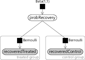
It is perfectly possible that a subject could recover from the illness without any medical intervention (or with a medical intervention that does nothing). In this model, we assume that the drug has no effect and therefore all recoveries are of this kind. We do not know what the probability of such a spontaneous recovery is and so we can introduce a random variable probRecovery to represent it, with a uniform Beta(1,1) prior. Then for each variable in the recoveredControl and recoveredTreated arrays, we assume that they were drawn from a Bernoulli distribution whose parameter is probRecovery. The resulting model is shown as a factor graph in Figure 6.9 – for a refresher on Beta-Bernoulli models like this one, take a look back at Chapter 2.
|
Model where the drug did have an effect
Now let’s turn to the second process, where the drug did have an effect on whether the patient recovered. In this case, we need to assume that there is a different probability of recovery for the treated group and for the control group. We hope that there is a higher probability of recovery for the treated group, but we are not going to assume this. We are only going to assume that the probability of recovery changes if the drug is taken.
- The probability of recovery is different for subjects in the treated group and for subjects in the control group.
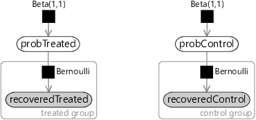
To encode this assumption in a factor graph, we need two variables: probTreated which is the probability of recovery for subjects who were given the drug and probControl which is the probability of recovery for subjects in the control group who were not given the drug. Once again, we choose uniform Beta(1,1) priors over each of these variables. Then for each variable in the recoveredControl array we assume that they were drawn from a Bernoulli distribution whose parameter is probControl. Conversely, for each variable in the recoveredTreated array we assume that they were drawn from a Bernoulli distribution whose parameter is probTreated. The resulting model is shown in Figure 6.10.
|
Compare the models of the two different processes given in Figure 6.9 and Figure 6.10. You can see that the factor graphs are pretty similar. The only difference is that the ‘no effect’ model has a single shared probability of recovery whilst the ‘has effect’ model has different probabilities of recovery for the treated and control groups.
Selecting between the two models
We now need to decide which of these two models gave rise to the actual outcomes measured in the trial. The task of choosing which of several models best fits a particular data set is called model selection. In model-based machine learning, if we want to know the value of an unknown quantity, we introduce a random variable for that quantity and infer a posterior distribution over the value of the variable. We can use exactly this approach to do model selection. Let’s consider a random variable called model which has two possible values NoEffect if the ‘no effect’ model gave rise to the data and HasEffect if the ’has effect’ model gave rise to the data. Notice the implicit assumption here:
- Either the ‘no effect’ model or the ‘has effect’ model gave rise to the data. No other model will be considered.
For brevity, let’s use data to refer to all our observed data, in other words, the two arrays recoveredTreated and recoveredControl. We can then use Bayes’ rule (Panel 1.1) to infer a posterior distribution over model given the data.

Models can be compared using model evidence, in a process called Bayesian model selection.
Unsurprisingly, this technique of using Bayes’s rule to do model selection is called Bayesian model selection. In equation (6.1), the left hand side is the posterior distribution over models that we want to compute. On the right hand side, encodes our prior belief about which model is more probable – usually, this prior is chosen to be uniform so as not to favour any one model over another. Also on the right hand side, gives the probability of the data conditioned on the choice of model. This is the data-dependent term that varies from model to model and so provides the evidence for or against each model. For this reason, this quantity is known as the model evidence or sometimes just as the evidence.
With a uniform prior over models, the result is that the posterior distribution over model is equal to the model evidence values normalised to add up to 1. In other words, the posterior probability of a model is proportional to the model evidence for that model. For this reason, when comparing two models, it is common to look at the ratio of their model evidences – a quantity known as a Bayes factor. For example, the Bayes factor comparing the ‘has effect’ model evidence to the ‘no effect’ model evidence is:
The higher the Bayes factor, the stronger the evidence that the top model (in this case the ’has effect’ model) is a better model than the bottom model (the ’no effect’ model). For example, Kass and Raftery [1995] suggest that a Bayes factor between 3-20 is positive evidence for the top model, a Bayes factor between 20-150 is strong evidence, and a Bayes factor above 150 is very strong evidence. However, it is important to bear in mind that this evidence is only relative evidence that the top model is better than the bottom one – it is not evidence that this is the true model of the data or even that it is a good model of the data.
You might worry that the ‘has effect’ model will always be favoured over the ‘no effect’ model, because the ‘has effect’ model includes the ‘no effect’ model as a special case (when probTreated is equal to probControl). This means that the ‘has effect’ model can always fit any data generated by the ‘no effect’ model. So, even if the drug has no effect, the ‘has effect’ model will still fit the data well. As we will see when we start computing Bayes factors, if the drug has no effect the Bayes factor will correctly favour the ‘no effect’ model.
So why is the ‘no effect’ model favoured in this case? It is because of a principle known as Occam's razor (named after William of Ockham who popularized it) which can be expressed as “where multiple explanations fit equally well with a set of observations, favour the simplest”. Bayesian model selection applies Occam’s razor automatically by favouring simple models (generally those with fewer variables) over complex ones. This arises because a more complex model can generate more different data sets than a simpler model, and so will place lower probability on any particular data set. It follows that, where a data set could have been generated by either model, it will have higher probability under the simpler model – and so a higher model evidence. We will see this effect in action in the next section, where we show how to compute model evidences and Bayes factors for different trial outcomes.
Comparing the two models using Bayesian model selection
In this optional section, we show the inference calculations needed to do Bayesian model selection for the two models we just described. If you want to focus on modelling, feel free to skip this section.
Next we can look at how to perform Bayesian model selection between the two models in our randomised controlled trial. As an example, we will consider a trial with 40 people: 20 in the control group and 20 in the treated group. In this example trial, we found that 13 out of 20 people recovered in the treated group compared to just 8 out of 20 in the control group. To do model selection for this trial, we will need to compute the model evidence for each of our two models.
Computing the evidence for the ‘no effect’ model
Let’s first compute the evidence for the ‘no effect’ model, which is given by . Remembering that data refers to the two arrays recoveredTreated and recoveredControl, we can write this more precisely as .
If we write down the joint probability for the ‘no effect’ model, it looks like this:
In equation (6.3), the notation means a product of all the contained terms where varies over all the people in the treated group. Notice that there is a term in the joint probability for each factor in the factor graph of Figure 6.9, as we learned back in section 2.1. Also notice that when working with multiple models, we write the joint probability conditioned on the choice of model, in this case . This conditioning makes it clear which model we are writing the joint probability for.
We can simplify this joint probability quite a bit. First, we can note that is a uniform distribution and so we can remove it (because multiplying by a uniform distribution has no effect). Second, we can use the fact that recoveredTreated and recoveredControl are both observed variables, so we can replace the Bernoulli terms by for each subject that recovered and by for each subject that did not recover. It is helpful at this point to define some counts of subjects. Let’s call the number of treated group subjects that recovered and the number which did not recover . Similarly, let’s call the number of control group subjects that recovered and the number which did not recover .
This joint probability is quite similar to the model evidence that we are trying to compute . The difference is that the joint probability includes the probRecovery variable. In order to compute the model evidence, we need to remove this variable by marginalising (integrating) it out.
To evaluate this integral, we can compare it to the probability density function of the beta distribution, that we introduced back in equation (2.22):
We know that the integral of this density function is 1, because the area under any probability density function must be 1. Our model evidence in equation (6.5) looks like the integral of a beta distribution with and , except that it is not being divided by the normalising beta function . If we did divide by , the integral would be 1. Since we are not, the integral must equal for the above values of and . In other words, the model evidence is equal to .
For the counts in our example, this model evidence is , which equals .
Computing the evidence for the ‘has effect’ model
The computation of the model evidence for the ‘has effect’ model is actually quite similar. Again, we write down the joint distribution
We now condition the joint distribution on , which shows that this is the joint distribution for the ‘has effect’ model. We can simplify this expression by removing the uniform beta distributions and again using the counts of recovered/not recovered subjects in each group:
Notice that in this model we have two extra variables that we need to get rid of by marginalisation: probTreated and probControl. To integrate this expression over these extra variables, we can use the same trick as before except that now we have two beta densities: one over probTreated and one over probControl. The resulting model evidence is:
For the counts in our example, this model evidence is , which simplifies to .
Computing the Bayes factor for the ‘has effect’ model over the ‘no effect’ model
We now have the model evidence for each of our two models:
These model evidence values can be plugged into equation (6.1) to compute a posterior distribution over the model variable.
Let’s compute the Bayes factor for our example trial, where 8/20 of the control group recovered, compared to 13/20 of the treated group:
A Bayes factor of just 1.25 shows that the ’has effect’ model is very slightly favoured over the ’no effect’ model but that the evidence is very weak. Note that this does not mean that the drug has no effect, but that we have not yet shown reliably that it does have an effect. The root problem is that the trial is just too small to provide strong evidence for the effect of the drug. We’ll explore the effect on the Bayes factor of increasing the size of the trial in the next section.
Earlier, we claimed that the Bayes factor will correctly favour the ‘no effect’ model in the case where the drug really has no effect. To prove this, let’s consider a trial where the drug does indeed have no effect, which leads to an outcome of 8/20 recovering in both the control and treated groups. In this case, the Bayes factor is given by:
Now we have a Bayes factor of less than 1 which means that the ‘no effect’ model has been favoured over the ‘has effect’ model, despite them both fitting the data equally well. This tendency of Bayesian model selection to favour simpler models is crucial to selecting the correct model in real applications. As this example shows, without it, we would not be able to tell that a drug doesn’t work! For more explanation of this preference for simpler, less flexible models take a look at section 7.3 in the next chapter.
The model evidence calculations we have just seen have a familiar form. We introduced a random variable called model and then used Bayes’ rule to infer the posterior distribution over that random variable. However, the random variable model did not appear in any factor graph and we manually computed its posterior distribution, rather than using a general-purpose message passing algorithm. It would be simpler, easier and more consistent if the posterior distribution could be calculated by defining a model containing the model variable and running a standard inference algorithm on that model. In the next section, we show that this can be achieved using a modelling structure called a gate.
randomised controlled trialA randomised controlled trial is a kind of clinical trial commonly used for testing the effectiveness of various types of medical intervention, such as new drugs. In such a trial, each subject is randomly assigned into either a treated group (which receives the experimental intervention) or a control group (which does not receive the intervention). The purpose of the trial is to determine whether the experimental intervention has an effect or not on one or more outcomes of interest, and to understand the nature of that effect.
model selectionThe task of choosing which of several models best fits a particular data set. Model selection is helpful not only because it allows the best model to be used, but also because identifying the best model helps to understand the processes that gave rise to the data set.
Bayesian model selectionThe process of doing model selection by computing a posterior distribution over the choice of model conditioned on a given data set. Rather than given a single ‘best’ model, Bayesian model selection returns a probability for each model and the relative size of these probabilities can be used to assess the relative quality of fit of each model.
model evidenceThe probability of the data conditioned on the choice of model, in other words . This conditional probability provides evidence for or against each model being the one that gave rise to the data set, thus the name ‘model evidence’. Comparing model evidence values for different models allows for Bayesian model selection. Because it is a frequently used concept, model evidence is often called just the ‘evidence’.
Bayes factorThe ratio of the model evidence for a particular model of interest to the model evidence for another model, usually a baseline or ‘null’ model. The higher the Bayes factor, the greater the support for the proposed model relative to the a baseline model.
Occam's razorWhere multiple explanations fit equally well with a set of observations, favour the simplest. It is named after William of Ockham who used it in his philosophical arguments. He did not invent the concept, however, there are references to it as early as Aristotle (384-322 BC).
[Kass and Raftery, 1995] Kass, R. E. and Raftery, A. E. (1995). Bayes factors. Journal of the American Statistical Association, 90(430):773–795.