1.3 A model of a murder

To solve the murder, we need to incorporate more evidence from the crime scene. Each new piece of evidence will add another random variable into our joint distribution. To manage this growing number of variables, we will now introduce the central concept of this book: the probabilistic model. A probabilistic model consists of:

• A set of random variables,
• A joint probability distribution over these variables (i.e. a distribution that assigns a probability to every configuration of these variables such that the probabilities add up to 1 over all possible configurations).

Once we have a probabilistic model, we can reason about the variables it contains, make predictions, learn about the values of some random variables given the values of others, and in general, answer any possible question that can be stated in terms of the random variables included in the model. This makes a probabilistic model an incredibly powerful tool for doing machine learning.

We can think of a probabilistic model as a set of assumptions we are making about the problem we are trying to solve, where any assumptions involving uncertainty are expressed using probabilities. The best way to understand how this is done, and how the model can be used to reason and make predictions, is by looking at example models. In this chapter, we give the example of a probabilistic model of a murder. In later chapters, we shall build a variety of more complex models for other applications. All the machine learning applications in this book will be solved solely through the use of probabilistic models.

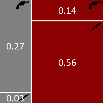
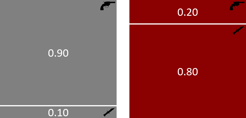
So far we’ve constructed a model of with two random variables: murderer and weapon. For this two-variable model, we were able to write the joint distribution pictorially, like so:

= $\times$ $P(\var{weapon}, \var{murderer})$   $P(\var{murderer})$   $P(\var{weapon} | \var{murderer})$

Figure 1.9The joint distribution for our two-variable model, shown as a product of two factors.

Unfortunately, if we increase the number of random variables in our model beyond two (or maybe three), we cannot represent the joint distribution using this pictorial notation. But in real models there will typically be anywhere from hundreds to hundreds of millions of random variables. We need a different notation to represent and work with such large joint distributions.

The notation that we will use exploits the fact that most joint distributions can be written as a product of a number of terms or factors each of which refers to only a small number of variables. For example, our joint distribution above is the product of two factors: $P(\var{murderer})$ which refers to one variable and $P(\var{weapon} | \var{murderer})$ which refers to two variables. Even for joint distributions with millions of variables, the factors which make up the distribution usually refer to only a few of these variables. As a result, we can represent a complex joint distribution using a factor graph [Kschischang et al., 2001] that shows which factors make up the distribution and what variables those factors refer to.

Figure 1.10 shows a factor graph for the two-variable joint distribution above. There are two types of node in the graph: a variable node for each variable in the model and a factor node for each factor in the joint distribution. Variable nodes are shown as white ellipses (or rounded boxes) containing the name of the variable. Factor nodes are small black squares, labelled with the factor that they represent. We connect each factor node to the variable nodes that it refers to. For example, the $P(\var{murderer})$ factor node is connected only to the $\var{murderer}$ variable node since that is the only variable it refers to, whilst $P(\var{weapon} | \var{murderer})$ connects to both the weapon and murderer variable nodes, since it refers to both variables. Finally, if the factor defines a distribution over one of its variables, we draw an arrow on the edge pointing to that variable (the child variable). If the factor defines a conditional distribution, the other edges from that factor connect to the variables being conditioned on (the parent variables) and do not have arrows.

bool variable The identity of the murderer (either Grey or Auburn). murderer int variable The murder weapon used (either dagger or revolver). weaponP(murderer)P(weapon|murderer)

Figure 1.10Factor graph for the murder mystery model. The model contains two random variables murderer and weapon, shown as white nodes, and two factors $P(\var{murderer})$ and $P(\var{weapon} | \var{murderer})$, shown as black squares.

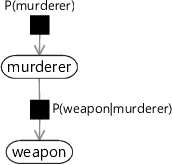
The factor graph of Figure 1.10 provides a complete description of our joint probability, since it can be found by computing the product of the distributions represented by the factor nodes. As we look at more complex factor graphs throughout the book, it will always hold that the joint probability distribution over the random variables (represented by the variable nodes) can be written as the product of the factors (represented by the factor nodes). The joint distribution gives a complete specification of a model, because it defines the probability for every possible combination of values for all of the random variables in the model. Notice that in Figure 1.9 the joint distribution was represented explicitly, but in the factor graph it is represented only indirectly, via the factors.

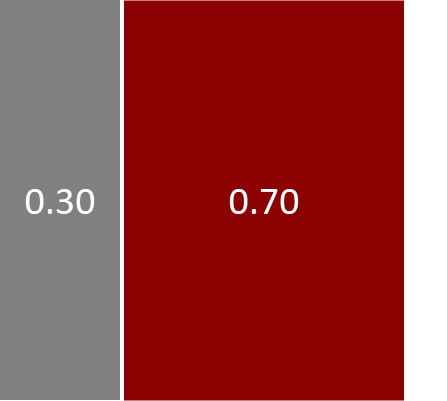
Since we want our factor graphs to tell us as much as possible about the joint distribution, we should label the factors as precisely as possible. For example, since we know that $P(\var{murderer})$ defines a prior distribution of $\dist{Bernoulli}(0.7)$ over murderer, we can label the factor “Bernoulli(0.7)”. We do not need to mention the murderer variable in the factor label since the factor is only connected to the murderer variable node, and so the distribution must be over murderer. This allows more informative labelling of the factor graph, like so:

bool variable The identity of the murderer (either Grey or Auburn). murderer int variable The murder weapon used (either dagger or revolver). weaponBernoulli(0.7)P(weapon|murderer)

Figure 1.11Factor graph representation of the murder mystery model with the Bernoulli prior over murderer labelled explicitly.

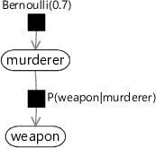
In this book, we will aim to label factors in our factor graphs so that the function represented by each factor is as clear as possible.

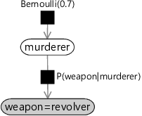
There is one final aspect of factor graph notation that we need to cover. When doing inference in our two-variable model, we observed the random variable weapon to have the value revolver. This step of observing random variables is such an important one in model-based machine learning that we introduce a special graphical notation to depict it. When a random variable is observed, the corresponding node in the factor graph is shaded (and sometimes also labelled with the observed value), as shown for our murder mystery in Figure 1.12.

observed bool variable The murder weapon used (either dagger or revolver). weapon=revolver bool variable The identity of the murderer (either Grey or Auburn). murdererBernoulli(0.7)P(weapon|murderer)

Figure 1.12The factor graph for the murder mystery, with the weapon node shaded to indicate that this random variable has been observed, and is fixed to the value revolver.

Representing a probabilistic model using a factor graph gives many benefits:

• It provides a simple way to visualize the structure of a probabilistic model and see which variables influence each other.
• It can be used to motivate and design new models, by making appropriate modifications to the graph.
• The assumptions encoded in the model can be clearly seen and communicated to others.
• Insights into the properties of a model can be obtained by operations performed on the graph.
• Computations on the model (such as inference) can be performed by efficient algorithms that exploit the factor graph structure.

We shall illustrate these points in the context of specific examples throughout this book.

Inference without computing the joint distribution

Having observed the value of weapon, we previously computed the full joint distribution and used it to evaluate the posterior distribution of murderer. However, for most real-world models it is not possible to do this, since the joint distribution would be over too many variables to allow it to be computed directly. Instead, now that we have our joint distribution represented as a product of factors, we can arrive at the same result by using only the individual factors – in a way which is typically far more efficient to compute. The key lies in applying the product and sum rules of probability in an appropriate way. From the product rule (1.15) we have

However, by symmetry we can equally well write

Equating the right-hand sides of these two equations and re-arranging we obtain

This is an example of Bayes' theorem or Bayes’ rule [Bayes, 1763] which plays a fundamental role in many inference calculations (see Panel 1.1). Here $P(\var{murderer})$ is the prior probability distribution over the random variable murderer and is one of the things we specified when we defined our model for the murder mystery. Similarly, $P(\var{weapon} | \var{murderer})$ is also something we specified, and is called the likelihood function and should be viewed as a function of the random variable murderer. The quantity on the left-hand side $P(\var{murderer} | \var{weapon})$ is the posterior probability distribution over the murderer random variable, i.e. the distribution after we have observed the evidence of the revolver.

The denominator $P(\var{weapon})$ in equation (1.24) plays the role of a normalization constant and ensures that the left hand side of Bayes’ theorem is correctly normalized (i.e. adds up to 1 when summed over all possible states of the random variable murderer). It can be computed from the prior and the likelihood using

which follows from the product and sum rules. When working with Bayes’ rule, it is sometimes useful to drop this denominator $P(\var{weapon})$ and instead write

where $\propto$ means that the left-hand side is proportional to the right-hand side (i.e. they are equal up to a constant that does not depend on the value of murderer). We do not need to compute the denominator because the normalization constraint tells us that the conditional probability distribution $P(\var{murderer} | \var{weapon})$ must add up to one across all values of murderer. Once we have evaluated the right hand side of (1.26) to give a number for each of the two values of murderer, we can scale these two numbers so that they sum up to one, to get the resulting posterior distribution.

Now let us apply Bayes’ rule to the murder mystery problem. We know that weapon=revolver, so we can evaluate the right hand side of equation (1.26) for both murderer=Grey and murderer=Auburn giving:

These numbers sum to 0.41. To get probabilities, we need to scale both numbers to sum to 1 (by dividing by 0.41) which gives:

This is the same result as before. Although we have arrived at the same result by a different route, this latter approach using Bayes’ theorem is preferable as we did not need to compute the joint distribution. With only two random variables so far in our murder mystery this might not look like a significant improvement, but as we go to more complex problems we will see that successive applications of the rules of probability allows us to work with small sub-sets of random variables – even in models with millions of variables!

factor graphA representation of a probabilistic model which uses a graph with factor nodes (black squares) for each factor in the joint distribution and variable nodes (white, rounded) for each variable in the model. Edges connect each factor node to the variable nodes that it refers to.

For example, here is a factor graph from Chapter 1:

bool variable The identity of the murderer (either Grey or Auburn). murderer int variable The murder weapon used (either dagger or revolver). weaponP(murderer)P(weapon|murderer)