1.4 Extending the model

Dr Bayes pulls out her trusty magnifying glass and continues her investigation of the crime scene. As she examines the floor near Mr Black’s body she discovers a hair lying on top of the pool of blood. “Aha” exclaims Dr Bayes “this hair must belong to someone who was in the room when the murder took place!” Looking more closely at the hair, Dr Bayes sees that it is not the lustrous red of Miss Auburn’s vibrant locks, nor indeed the jet black of the victim’s hair, but the distinguished silver of Major Grey!

Now that we are equipped with the concept of factor graphs, we can extend our model to incorporate this additional clue from the crime scene. The hair is powerful evidence indicating that Major Grey was present at the time of the murder, but there is also the possibility that the hair was stolen by Miss Auburn and planted at the crime scene to mislead our perceptive sleuth. As before, we can capture these thoughts quantitatively using a conditional probability distribution. Let us denote the new information by the random variable hair, which takes the value true if Major Grey’s hair is discovered at the scene of the crime, and false otherwise. Clearly the discovery of the hair points much more strongly to Grey than to Auburn, but it does not rule out Auburn completely.

Suppose we think there is a 50% chance that Grey would accidentally leave one of his hairs at the crime scene if he were the murderer, but that there is only a 5% chance that Auburn would think to plant a grey hair if she were the murderer. The conditional probability distribution would then be

As we have seen before, this is the conditional probability of hair being true given two different values of murderer, not a probability distribution over hair, and so the numbers in (1.32) do not have to add up to one.

In writing the conditional probability this way, we have actually made an additional assumption: that the probability of one of Major Grey’s hairs being found at the scene of the crime only depends on who committed the murder, and not anything else – including the choice of weapon that was used to commit the murder. This assumption has arisen because the conditional probability in (1.32) does not include weapon in the variables being conditioned on. Mathematically this assumption can be expressed as

which says that the distribution of hair is independent of the value of weapon once we have conditioned on the value of murderer. For this reason it is known as a conditional independence assumption. Notice that (1.33) has a similar form to the equations which hold when two variable are independent, e.g. (1.12), but has an additional conditioning variable on both sides.

The question to ask when considering a conditional independence assumption is “Does learning about one variable, tell me anything about the other variable, if I knew the value of the conditioning variable?”. In this case that would be “Does learning about the hair, tell me anything about the choice of weapon, if I already knew who the murderer was?”. Reasonably, the answer in this case might be that you could learn a little (for example, the dagger might mean the murderer had to get closer to the victim and so was more likely to drop a hair). However, for the sake of simplicity we assume that this conditional independence assumption holds.

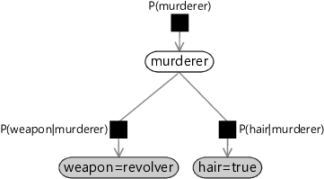
Figure 1.13 shows the factor graph corresponding to our expanded model with the new hair variable and a new factor representing this conditional distribution. Our conditional independence assumption has a simple graphical interpretation, namely that there is no edge connecting the weapon node directly to the factor representing the conditional distribution $P(\var{hair}|\var{murderer})$. The only way to get from the weapon node to the hair node is via the murderer node. We see that the missing edges in the factor graph capture independence assumptions built into the model.

observed bool variable The murder weapon used (either dagger or revolver). weapon=revolver observed bool variable Whether or not a grey hair is present at the crime scene. hair=true bool variable The identity of the murderer (either Grey or Auburn). murdererP(murderer)P(weapon|murderer)P(hair|murderer)

Figure 1.13The factor graph for the murder mystery after the addition of the new evidence. Both the weapon node and the hair node are shaded to indicate that these random variables have been set to their observed values. Note the absence of an edge connecting the weapon random variable with the factor node representing $P(\var{hair}|\var{murderer})$.

There is an alternative graphical representation of a model called a Bayesian network or Bayes net that emphasises such independence assumptions, at the cost of hiding information about the factors. It provides less detail about the model than a factor graph, but gives a good ‘big picture’ view of which variables directly and indirectly affect each other. See Panel 1.2 for more details.

Panel 1.2Bayesian Networks

A Bayesian network is a different way of using a graph to represent a probabilistic model [Pearl, 1985; Pearl, 1988]. In a Bayes net, there are variable nodes corresponding to each variable in the model, but there are no factor nodes. Parent variables of a factor are connected directly to the child variable of the factor, using directed edges (arrows). For example, the Bayes net corresponding to the factor graph of our murder (Figure 1.13) looks like this:

observed bool variable The murder weapon used (either dagger or revolver). weapon=revolver observed bool variable Whether or not a grey hair is present at the crime scene. hair=true bool variable The identity of the murderer (either Grey or Auburn). murderer

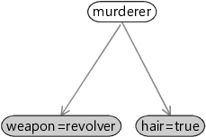
As this figure shows, by hiding the factors, a Bayes net emphasises which variables there are and how they influence each other (directly or indirectly). Bayes nets can be very useful in the early stages of model design when you want to focus on what variables to include and which will affect each other, without yet getting into details of precisely how they affect each other.

The disadvantage of using a Bayes net is that it is an incomplete specification of a model – you also have to write down all the factor functions externally to the graph and consider the two together as making up the model. For this reason, we have chosen to use factor graphs in this book, since they provide a stand-alone description of the model.

Given the factor graph of Figure 1.13, we can write down the joint distribution as the product of three terms, one for each factor in the factor graph:

Check for yourself that each term on the right of equation (1.34) corresponds to one of the factor nodes in Figure 1.13.

Incremental inference

We want to compute the posterior distribution over murderer in this new model, given values of weapon and hair. Given that we have the result from the previous model, we’d like to make use of it – rather than start again from scratch. To get our posterior distribution in the previous model, we conditioned on the value of weapon. To perform incremental inference in this new model, we can write down Bayes’ rule but condition each term on the variable weapon:

We can use exactly the same trick as we did back in equation (1.26) to drop the denominator and replace the equals sign with a proportional sign $\propto$:

Remembering that hair and weapon are conditionally indepedent given murderer, we can use equation (1.33) and drop weapon from the last term:

Since we know the values of weapon and hair, we can write in these observations:

We can now compute the new posterior distribution for murderer. As before, each term depends only on the value of murderer and the overall normalization can be evaluated at the end. Substituting in the posterior we obtained in section 1.2 and our new conditional probability from equation (1.32) gives:

The sum of these two numbers is 0.347, and dividing both numbers by their sum we obtain the normalized posterior probabilities in the form

Taking account of all of the available evidence, the probability that Grey is the murderer is now 95%.

As a recap, we can plot how the probability distribution over murderer changed over the course of our murder investigation (Figure 1.14). Notice how the probability of Grey being the murderer started out low and increased as each new piece of evidence stacked against him. Similarly, notice how the probability of Auburn being the murderer evolved in exactly the opposite direction, due to the normalization constraint and the assumption that either one of the two suspects was the murderer. We could seek further evidence, in the hope that this would change the probability distribution to be even more confident (although, of course, evidence implicating Auburn would have the opposite effect). Instead, we will stop here – since 95% is greater than our threshold of 91% and so enough for a conviction!

Excel

CSV

Figure 1.14The evolution of $P(murderer)$ over the course of the murder investigation.

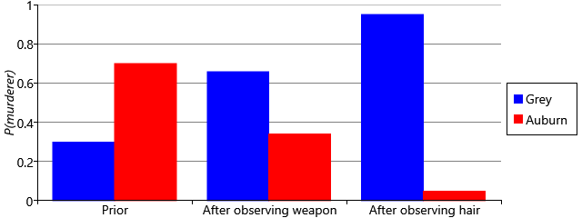
The model of the murder that we built up in this chapter contains various prior and conditional probabilities that we have set by hand. For real applications, however, we will usually have little idea of how to set such probability values and will instead need to learn them from data. In the next chapter we will see how such unknown probabilities can be expressed as random variables, whose values can be learned using the same probabilistic inference approach that we just used to solve a murder.

Bayesian networkA graphical model where nodes correspond to variables in the model and where edges show which variables directly influence each other. Factors are not shown, but the parent variables in a factor are connected directly to the child variable, using directed edges (arrows). See Panel 1.2.

For example, here is a Bayes net for the model of Chapter 1:

observed bool variable The murder weapon used (either dagger or revolver). weapon=revolver observed bool variable Whether or not a grey hair is present at the crime scene. hair=true bool variable The identity of the murderer (either Grey or Auburn). murderer

[Pearl, 1985] Pearl, J. (1985). Bayesian networks: A model of self-activated memory for evidential reasoning. In Proc. of Cognitive Science Society (CSS-7).