8.3 Principal Component Analysis

Principal component analysis (PCA) assumes that a data set arose from mixing together some underlying signals in different ways. PCA then attempts to ‘un-mix’ the data, so as to recover these original signals. More precisely, PCA is a procedure for transforming a set of observation of correlated variables into a set of uncorrelated variables called principal components. PCA was invented back in 1901 by the mathematician Karl Pearson [Pearson, 1901] and, since that time, has been rediscovered and reformulated by numerous people for a variety of applications in fields from mechanical engineering to meteorology.

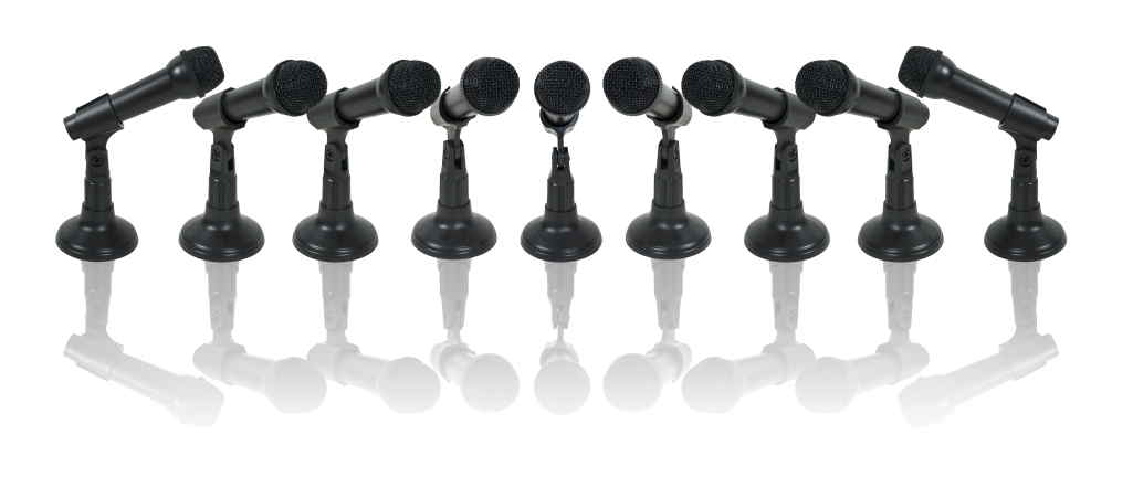
Multiple microphones will hear the same sounds but at different volumes.

The intent of applying PCA is usually to try to determine the underlying causes affecting a measured data set. For example, in speech recognition, it is important to be able to separate the sounds from different sources, such as different speakers or background sources of noise. An array of microphones will pick up sound from each source to a different extent, so the audio signals reaching the microphones will likely be correlated. To try and separate out the individual audio signals from different sources, someone may try to use a method like PCA, under the assumption that the individual sources are uncorrelated. Importantly, ‘uncorrelated’ in PCA means linearly uncorrelated – whilst there will be no linear dependency between the principal components, there may well remain a nonlinear dependency. We will see later that this definition of uncorrelated has significant implications in the behaviour of PCA.

Other applications of PCA include applying it to stock market data, to try and understand underlying causes that affect many stocks at once. PCA has also been used to process readings from correlated sensors, such as in neuroscience applications when sensing neural activation. More generally, PCA is used for visualizing high dimensional data – for example, by plotting only the largest few principal components, which are assumed to capture the most important aspects of the data.

Computing the principal components

In two dimensions, PCA can be thought of as fitting an ellipse to the data where each axis of the ellipse represents a principal component. This idea is illustrated in Figure 8.6.

Figure 8.6A visualization of the principal components of a two dimensional data set. If we fit an ellipse to our data, the axes of the ellipse give the directions of the principal components, as indicated by the red arrows.

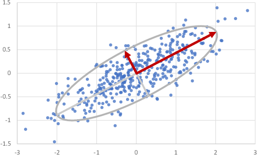
In $n>2$ dimensions, PCA can similarly be thought of as fitting an $n$-dimensional ellipsoid. The process for fitting the ellipsoid is:

1. Subtract the mean of each variable from each value to centre the data set at zero;
2. Compute the covariance matrix of the centered data set;
3. Calculate the principal components as the eigenvectors of this covariance matrix, as described in Bishop [2006], section 12.1.

When the number of dimensions is large, it is common for some axes of the fitted ellipsoid to become quite small. The corresponding principal directions have small variance and so can be collapsed without losing much information in the original signals. In our microphone array, for example, we might hope that collapsing directions with small variance would leave only those directions corresponding to distinct sources of sound – that is, each individual speaker, whilst reducing general background noise.

A factor graph for PCA

It is far from obvious how to construct a factor graph to get random variables corresponding to the principal components of a set of observed data. Happily, this task has already been done for us by Tipping and Bishop [1999], where the authors develop a probabilistic model which achieves exactly this. The factor graph for this model is shown in Figure 8.7. In this model, maximum likelihood inference of the weight matrix gives the principal components of the observed signal data.

plate of size: signals signals plate of size: components components plate of size: time time observed double[,] variable The measured value of this signal at this point in time. signal double[] variable The mean of this signal, across time. mean double[,] variable The value of this uncorrelated source at this point in time. source double[,] variable The amount that a particular source contributes to a particular signal. weight double[,] variable The reconstruction of this signal as a weighted sum of sources (principal components). weightedSum double variable The variance of the measurement noise. noiseVariance double variable The reconstruction of this signal shifted by the mean. shiftedGaussian(0,100)Gaussian(0,1)Gaussian(0,1)MatrixMultiply+Gaussian

Figure 8.7Factor graph for probabilistic principal component analysis.

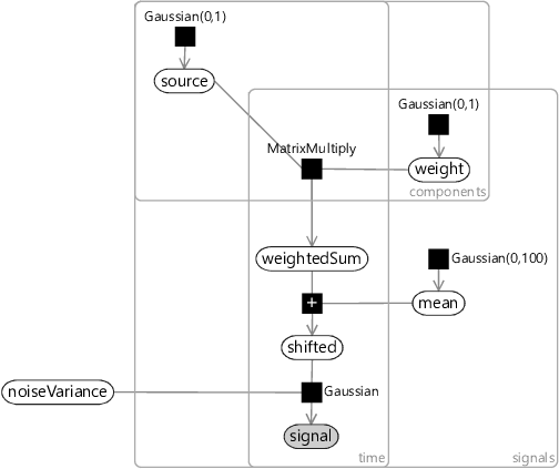
Let’s have a look at what’s going on in this factor graph. The graph contains three plates:

• The number of signals, such as the number of microphones in the microphone array;
• The number of components, the number of principal components to find;
• The number of data points, which we’ve called time since it is common for these to be measurements across time. However, they could be any set of measurements, such as measurements of pixels in an image.

The core idea of PCA is to transform the signal dimensions into a smaller number of underlying principal component directions. We can see this in the coarse structure of the graph – the observed signal and most variables near it live in the signals plate, but further up the graph the variables lie in the components plate. More specifically, we start at the top with a variable for the uncorrelated source components which, unsurprisingly, lies in the components plate. The weight variable is the only one in both the components and signals plates and it is responsible for transforming between the two. The weightedSum variable holds a weighted sum of components that approximately reconstructs the centered signal. This is then ‘un-centered’ by shifting it by the mean to get the shifted form. Finally, we add noise with variance noiseVariance to give the observed signal. This noise accounts for differences between the reconstruction and the actual measured signal.

In Figure 8.7, we have chosen Gaussian(0,1) priors for the uncorrelated source components and the elements of the weight matrix. This assumes that the signals have approximately unit variance – in other words, that the signal variation is on the order of $\pm1$. If this is not the case, then it is common to re-scale the signal before applying PCA – for example, to ensure it has unit variance. Because we are using a probabilistic model, we have the option of changing the priors instead – for example, by making the source components have a prior matched to the observed signal. The factor graph also shows a broad Gaussian(0,100) prior for the mean. This prior assumes that the mean lies somewhere roughly in the range $0\pm10$ on each dimension. With PCA it is common to subtract the mean – but with this model you do not have to as long as the prior on mean is sufficiently broad to include the actual mean of the data.

Representing PCA as a probabilistic model allows us to use standard inference algorithms to infer the principal components. This can be useful in situations where the normal algorithm cannot be applied. For example, if there is missing data, we cannot compute the covariance matrix and so the normal PCA algorithm cannot be used. However, in the probabilistic model, an inference algorithm can still be run when some of the signal variables are not observed. We can even use the inference algorithm to compute posterior distributions over such unobserved variables to fill in missing values!

The assumptions built in to PCA

With the factor graph for PCA in hand, we can now read off the assumptions being made. As before, we’ll start at the bottom with the observed signal variable. We are assuming that this observation consists of an underlying component coming from the shared sources (shifted) and some signal-specific variability which we are modelling as Gaussian measurement noise. So our first assumption is:

1. The measurement noise is Gaussian.

For some kinds of sensors, the noise really is approximately Gaussian, and so this will be a perfectly fine assumption. The problem comes if the sensor noise is non-Gaussian and occasionally gives large noise values, which will show up as outliers in the data. Since the PCA model assumes that there are no outliers, these will be assumed to be valid data points and will strongly affect the inferred principal components. Informally, they will drag the fitted ellipsoid toward the outlier – not a good thing!

Moving up the graph, we get to where the weightedSum is being reconstructed by multiplying the underlying source components by the weight matrix. This is where the really interesting assumptions are being made, starting with:

2. All underlying sources affect all signals.

Elements in the weight matrix have a Gaussian(0,1) prior, which does not encourage the elements to be zero or near-zero. As a result, we may expect weights to be generally non-zero and so every source will have an effect on every signal. For our microphone array, this may be a perfectly reasonable assumption. The microphones are close together and we might expect that any sound source heard by one of the microphones would be audible to the other microphones. In other settings, however, this assumption may not be so reasonable. For example, if modelling stock prices, we might expect certain underlying events to only affect stocks in a particular industry, but to have almost no effect at all on stocks in other industries. The PCA model would likely fail to capture such a localized effect.

An event may cause one stock to go up, but another to go down.

Another assumption about the weight matrix is:

3. Weights can be positive or negative.

In some applications, we may want the weights to represent the degree to which a source affects a particular signal. For example, in a microphone array we want the weights to represent how loud the source signal is at each microphone. In such cases, it only makes sense for the weights to be positive, since there is no physical mechanism for inverting the effect of the source. When modelling stock prices, however, it is perfectly reasonable to assume that some underlying event has a positive effect on some stocks and a negative effect on others. For example, the outbreak of a pandemic may cause video conference stocks to rise but airline stocks to fall. The result of incorrectly allowing negative weights is that the inferred source signals may get inverted. In addition, it introduces a symmetry in the model which can cause problems during inference, as discussed in section 5.3.

A related assumption is:

4. Sources can be positive or negative.

As with the previous assumption, there are applications where it makes sense for the underlying sources to be positive or negative (such as when they are audio signals) and applications where it does not (such as where the underlying causes are events). As before, getting this assumption wrong can lead to symmetries that make inference problematic.

We’ll look at one more assumption, which turns out to be quite critical:

5. Sources are Gaussian-distributed.

This assumption is critical in order for the model to discover uncorrelated principal components. Because principal directions are orthogonal (at right angles to each other), this means that the rows of the weight matrix will be orthogonal. This causes a major problem in many applications. For example, in our microphone array we might expect the rows in the weight matrix to be similar for nearby microphones. However, they cannot be similar if they need to be at right angles to each other!

(a)A sample data set

  

(b)Principal components

Figure 8.8(a) A sample data set where the underlying signals are picked up by different amounts in two sensors. Here, the weight matrix is non-orthogonal and so the direction of variation of the two signals are not at right angles. (b) Since PCA assumes Gaussian sources, it will always find principal directions which are at right angles, even if these do not match the underlying signals in the data.

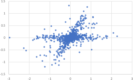
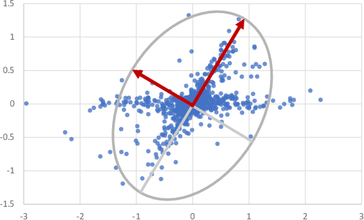
Figure 8.8 illustrates this problem. In this figure, data from two non-Gaussian sources has been mixed using a non-orthogonal weight matrix, much as might happen when two sound signals arrive at a nearby pair of microphones. Figure 8.8b shows the principal components of this data set, which are required to be at right angles to each other and so do not capture the directions of the underlying sources. Simply put, this assumption often makes PCA unusable – we instead have to use extensions to PCA that make different assumptions about the sources.

Extensions to PCA

PCA is such a well-known and useful method that people have extended it to fix the problems caused by each of the above assumptions. For example, to overcome issues caused by Assumptions0 8.1, robust PCA methods have been developed that infer the principal components reliably, even in the presence of outliers. Such robustness can be achieved by changing the measurement noise to be non-Gaussian. For example, Luttinen et al. [2012] use a distribution called a Student-t distribution to model the noise. This distribution has more probability mass in its tails than a Gaussian distribution and so is much more robust to outliers.

Assumptions0 8.2 is not appropriate for applications where measured signals will be affected by only some of the underlying sources. In such cases, variants of sparse PCA have been created which allow the weight matrix to contain many zero elements – see, for example, Tipping [2001].

In applications where the sources and weights are known to be positive (or zero), it is preferable to avoid Assumptions0 8.3 and Assumptions0 8.4. Here, non-negative matrix factorization (NMF) methods can be applied instead. These methods constrain the weights and sources to be non-negative. For example, NMF can be achieved by changing the priors on weight and source to distributions that only allow non-negative values. It follows that the prior on source must now be non-Gaussian and so Assumptions0 8.5 no longer holds, allowing for non-orthogonal weight matrices. Indeed, NMF does lead to a weight matrices with non-orthogonal rows.

We may want to have a non-orthogonal weight matrix without constraining our sources to be non-negative. To achieve this we can use some form of independent component analysis (ICA), which aims to infer latent sources that are not just linearly uncorrelated but actually statistically independent of each other. One way to do ICA is to change the prior over the source variable to a suitable non-Gaussian prior, thus changing Assumptions0 8.5. For example, the prior can be a mixture of Gaussians, as in Chan et al. [2003].

(a)PCA

  

(b)ICA

Figure 8.9Illustration of the difference between PCA and ICA. (a) As we saw in Figure 8.8, PCA will always find principal directions which are at right angles, since it assumes Gaussian sources. (b) ICA instead allows for sources to be non-Gaussian and so can recover the true directions of the sources.

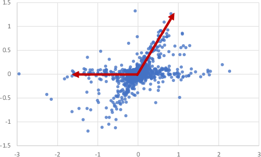
Figure 8.9 illustrates the difference in behaviour of ICA compared to PCA. As we saw in Figure 8.8, PCA finds principal directions at right angles (Figure 8.9a), whereas ICA discovers the underlying source directions, even though they are not orthogonal (Figure 8.9b). For our example task of separating out the different audio sources reaching a microphone array, ICA is clearly a better choice than PCA.