7.4 Communities of workers

In the previous section, our biased worker model failed to improve our accuracy, due to lack of data. More specifically, each worker does not have enough data for the model to learn a personalised conditional probability table to represent their biases. To consider how to solve this problem, think back to section 6.5 where we were learning how children gain or lose allergies. Rather than learning the probabilities of each individual child gaining or losing each allergy, we grouped the children into classes and learned probabilities for all children in a class. We can use exactly the same trick here!

It seems reasonable to group our workers together, as we may expect that there are communities of workers that have similar behaviour. We saw this when selecting worker confusion matrices for Figure 7.9 – many workers had very similar confusion matrices. For example, there seemed to be a community of workers who are very careful and give very good quality labels, another community who make mistakes about which tweets are relevant or not, a smaller community of workers who confuse the labels Neutral and Negative and so on. If we switch our model to learning conditional probability tables for whole communities, rather than for individual workers, then we will have much more data to train each CPT. More data will mean more certain inferred CPTs and so hopefully better accuracy. This was the approach taken by Venanzi et al. [2014] who developed a model very similar to the one we will now explore.

To change our model to learn CPTs for communities instead of workers, we need to modify our assumptions:

2. Each worker in a particular community will give a tweet a particular label with a worker community-specific probability that depends on the true label of the tweet.
3. Most workers communities will have a higher probability of giving the correct label than an incorrect one.

and add a new one:

4. Each worker belongs to a single community.

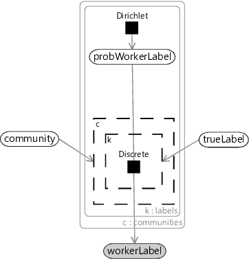
To encode these new assumptions in a model, we need to move the probWorkerLabel variable out of the plate over the workers and into a new plate over communities. Each worker will also need a new community variable to indicate which community that workers belongs to: 0, 1, 2 … and so on. We will need a new gate inside the communities plate which is switched on and off by this community variable. Given that we already have a gate connected to the trueLabel variable, this means that we now have two gates – one inside the other. The conditional probability for a label is therefore selected by both the community of the worker and the trueLabel of the tweet. Figure 7.15 shows the resulting factor graph for a single label with the two nested gates and the new community variable and plate.

plate of size: communities c : communities plate of size: labels k : labels gate (on when community=Var[c]) c gate (on when trueLabel=Var[k]) k observed int variable The label assigned to this tweet by this worker. workerLabel int variable The community that this worker belongs to. community int variable The true label for this tweet. trueLabel double[][][] variable An array of probabilities of a worker in this community giving a tweet each possible label, conditioned on the true label of the tweet. probWorkerLabelDirichletDiscrete

Figure 7.15Community model for a single label. The two nested gates show that the conditional probability for the worker label is selected by both the community of the worker and the trueLabel of the tweet.

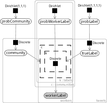
We expect some communities to be much larger than others, and so it will be useful to learn the probability that a worker belongs to each available community. We can use exactly the same approach as for learning the probability of each true label and create a new variable probCommunity that holds an array of probabilities that add up to 1 – and once again give this a Dirichlet prior. Putting everything together, gives us the overall model of Figure 7.16.

plate of size: tweets tweets plate of size: communities c : communities plate of size: labels k : labels plate of size: workers workers gate (on when community=Var[c]) c gate (on when trueLabel=Var[k]) k observed int[][] variable The label assigned to this tweet by this worker. workerLabel double[] variable An array of probabilities of a tweet having each possible label. probLabel double[] variable An array of probabilities of a worker belonging to each possible community. probCommunity int[] variable The community that this worker belongs to. community int[] variable The true label for this tweet. trueLabel double[][][] variable An array of probabilities of a worker in this community giving a tweet each possible label, conditioned on the true label of the tweet. probWorkerLabelDirichlet(1,1,1,1)Dirichlet(1,1,1)DiscreteDirichletDiscreteDiscrete

Figure 7.16The community model in full. Notice that this model has ended up having a symmetry between the two sides – the community variable and its parent probCommunity are connected just like the trueLabel variable and its parent probLabel.

Results of the community model

We can try out our model for different numbers of communities – say, between 1 and 3. For any of these, we can look at the inferred CPTs for each community given by the posterior over probWorkerLabel. These CPTs should give us a good understanding of the entire population of workers – what patterns of mistakes are made and how many workers fall into each pattern. For example, Figure 7.17 shows the inferred CPTs for a three-community model, along with the number of workers in the training set assigned to each community. The three CPTs show three different patterns of errors, much like the three example worker confusion matrices in Figure 7.9.

Excel

CSV

(a)CPT of the largest community with 842 workers

Excel

CSV

(b)CPT of the middle community with 561 workers

Excel

CSV

(c)CPT of the smallest community with 385 workers

Figure 7.17Learned conditional probability tables for our community model, run with three communities. Each CPT shows a different crowd worker bias. For example, the top CPT shows a community of workers which tend to label tweets incorrectly as Neutral – this bias is visible in the second column of the CPT where there is a relatively high probability of giving the label Neutral for the three rows where the true label is not Neutral. Similarly, the bottom CPT shows a community of workers that tend to label tweets incorrectly as Unrelated.

Understanding the kinds of mistakes different workers make can be useful by itself. For example, it provides insights in how to improve the training given to the workers. In our case, Figure 7.9 suggests that we should have additional training to show what tweets should be labelled as Neutral or Unrelated perhaps by showing workers real examples of tweets that have been incorrectly labelled. Hopefully, these kind of changes alone would lead to improvements in labelling accuracy. We could even provide customised training for each worker, tailored to the community that the worker belongs to!

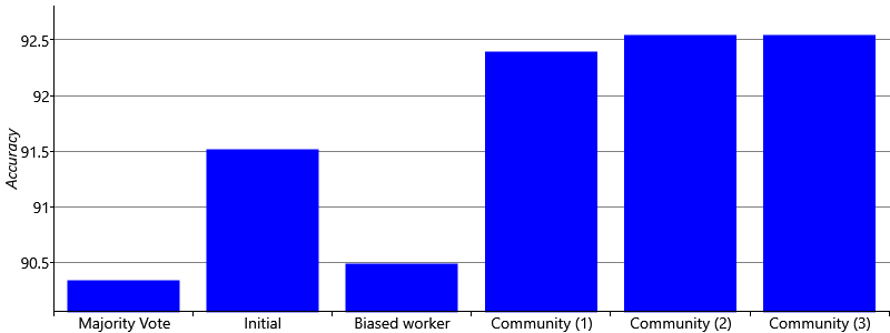
Even without improved worker training, now that we are modelling the error patterns of our workers, we may hope for improved accuracy. The accuracies for models with 1, 2 and 3 communities are shown in Figure 7.18, compared to the accuracies of previous models. The chart shows that our community model is now leading to improved accuracy, whether we choose 1, 2 or 3 communities. Interestingly, the numbers of communities does not seem to have much affect on the overall accuracy. This may be because the communities are similar enough that modelling one big community really well is nearly as good as modelling communities separately. It is also possible that having more communities means that there is less data per community and so more uncertainty in each community CPT. This uncertainty could be negatively affecting the accuracy.

Excel

CSV

Figure 7.18Accuracies for community models with 1, 2 and 3 communities, along with previous models for comparison. The community model is giving a good improvement in accuracy over the previous models. Surprisingly, having more communities does not seem to help the accuracy much.

Results with less training data

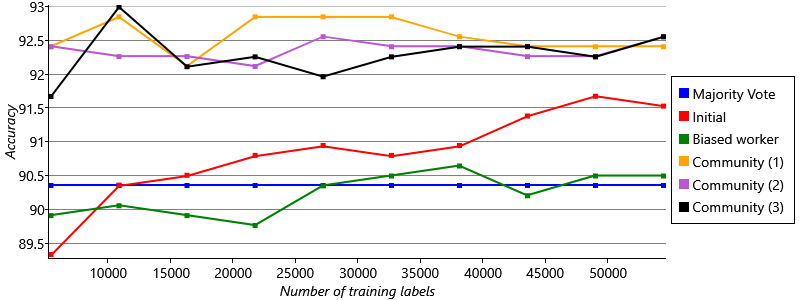
We’ve seen that our new community model works better than our previous models, and we believe this is because it makes better use of the available training data. In our application, we care deeply about how quickly we can get accurate labels – we want our system to be as accurate as possible even early on when there are relatively few labelled tweets. We can check how well our system performs with little training data by artificially reducing the size of our training set and seeing what effect this has on our accuracy. To do this, we will use training sets ranging from 10% of the original size up to 100% of the original size, in 10% increments. Figure 7.19 shows how the accuracy of each model varies as we increase the amount of training data.

Excel

CSV

Figure 7.19Plot showing how the accuracy of each model varies with the number of training labels. As the training data is reduced to 10% of its original size, the community models show only a small reduction in accuracy. In contrast, the accuracy of both the initial model and the biased worker model drop to below that of majority vote. As a result the communities models do even better than the other models when there are few training labels, since the gap is larger on the left of the plot than on the right.

The plot in Figure 7.19 is very encouraging for our community model. It shows that the accuracy of the model remains high even with only 10% of the training data (the left-hand end of the graph). This suggests that the model will do well early on, when there are relatively few labels, and also continue to give the best performance later, when more tweets have been labelled. Interestingly, we see that the initial model copes particularly badly with little training data: its accuracy drops rapidly as the training data is reduced and at 10% training data it is worse than both the biased worker model and the majority vote baseline! It seems we were very wise to move away from this model.

It is fantastic that our community model works well even when there are relatively few labels – but it would be even better if we could make our model useful before we have any labels at all! We will explore this idea in the next section.