-

Want a paper copy?
You can now buy the book!
All royalties go to the Cystic Fibrosis Trust.Spotted an error? Have comments?
Let us know!Get hands on with source code for the book.
2.3 Loopiness
Let’s now extend our model slightly by adding a fourth question which needs both skills. This new factor graph is shown in Figure 2.14, where we have added new isCorrect4 and hasSkills4 variables for the new question. Surely we can also do inference in this, very slightly larger, graph using belief propagation? In fact, we cannot.

Loops can be challenging.
The problem is that belief propagation can only send a message out of an (unobserved) node after we have received messages on all other edges of that node (Algorithm 2.1). Given this constraint, we can only send all the messages in a graph if there are no loops, where a loop is a path through the graph which starts and finishes at the same node (without using the same edge twice). If the graph has a loop, then we cannot send any of the messages along the edges of the loop because that will always require one of the other messages in the loop to have been computed first.
|
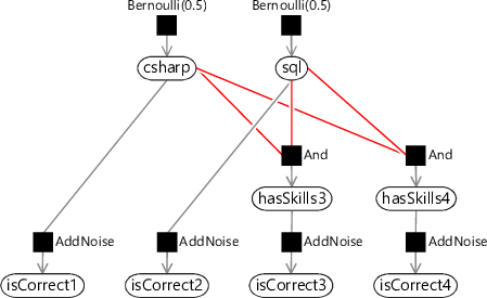
If you look back at the old three-question factor graph (Figure 2.5) you’ll see that it has no loops (a graph with no loops is called a tree) and so belief propagation worked without problems. However, our new graph does have a loop, which is marked in red in Figure 2.14. To do inference in such a loopy graph, we need to look beyond standard belief propagation.
To perform inference in loopy graphs, we need to get rid of the loops somehow. In this toy example, we could notice that hasSkills3 and hasSkills4 are the same and remove one of them. Such a simple solution is unlikely to be available in real problems. Instead, there are various general-purpose methods to remove loops, as described in Panel 2.2. Unfortunately, all these methods typically become too slow to use when dealing with large factor graphs. In most real applications the graphs are very large but inference needs to be performed quickly. The result is that such exact inference methods are usually too slow to be useful.
The alternative is to look at methods that compute an approximation to the required marginal distributions, but which can do so in much less time. In this book, we will focus on such approximate inference approaches, since they have proven to be remarkably useful in a wide range of applications. For this particular loopy graph, we will introduce an approximate inference algorithm called loopy belief propagation.
Loopy belief propagation
In this optional section, we define the loopy belief propagation algorithm and use it to perform inference in our loopy model. If you want to focus on modelling, feel free to skip this section.
Loopy belief propagation [Frey and MacKay, 1998] is identical to belief propagation until we come to a message that we cannot compute because it is in a loop. At that point, the loopy belief propagation algorithm computes the message anyway using a suitable initial value for any messages which are not yet available.
So, in loopy belief propagation, when we wish to compute a message that depends on other messages which are not yet computed, we use a special initial message value for the unavailable messages. This initial value is usually the uniform distribution (such as Bernoulli(0.5)) but in some cases it may be preferable to use some other user-supplied distribution. These initial message values allows us to break the loop and compute . Once we have computed , we will be able to compute other messages around the loop and eventually we get back to the original node. At this point, all the incoming messages needed to compute will have been computed, so we can recompute using these values instead of the initial ones. But because has changed in value, we can then go around the loop computing all the messages again. Which will bring us back to recomputing , and so on. After a number of iterations around the loop, this procedure often leads to the value of message not changing – we say that it has converged. At this point, we can stop sending any further messages, since there will be no further changes to the computed marginal distributions.
- Variable node message: the product of all messages received on the other edges;
- Factor node message: the product of all messages received on the other edges, multiplied by the factor function and summed over all variables except the one being sent to;
- Observed node message: a point mass at the observed value;
The complete loopy belief propagation algorithm is given as Algorithm 2.2 – it requires as input a message-passing schedule, which we will discuss shortly. Loopy belief propagation is not guaranteed to give the exactly correct result but it often gives results that are very close. Unlike exact inference methods, however, loopy belief propagation is still fast when applied to large models, which is a very desirable property in real applications.
Choosing a message-passing schedule
An important consequence of using loopy belief propagation is that we now need to provide a message-passing schedule, that is, we need to say the order in which messages will be calculated. This is in contrast to belief propagation where the schedule is fixed, since a message can be sent only at the point when all the incoming messages it depends on are received. A schedule for loopy belief propagation needs to be iterative, in that parts of it will have to be repeated until message passing has converged.
The choice of schedule can have a significant impact on the accuracy of inference and on the rate of convergence. Some guidelines for choosing a good schedule are:
- Message computations should use as few initial message values as possible. In other words, the schedule should be as close to the belief propagation schedule as possible and initial message values should only be used where absolutely necessary to break loops. Following this guideline will tend to make the converged marginal distributions more accurate.
- Messages should be sent sequentially around loops within each iteration. Following this guideline will make inference converge faster – if instead it takes two iterations to send a message around any loop, then the inference algorithm will tend to take twice as long to converge.
There are other factors that may influence the choice of schedule: for example, when running inference on a distributed cluster you may want to minimize the number of messages that pass between cluster nodes. Manually designing a message-passing schedule in a complex graph can be challenging – thankfully, there are automatic scheduling algorithms available that can produce good schedules for a large range of factor graphs, such as those used in Infer.NET [Minka et al., 2014].
Applying loopy belief propagation to our model
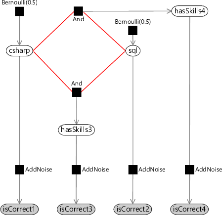
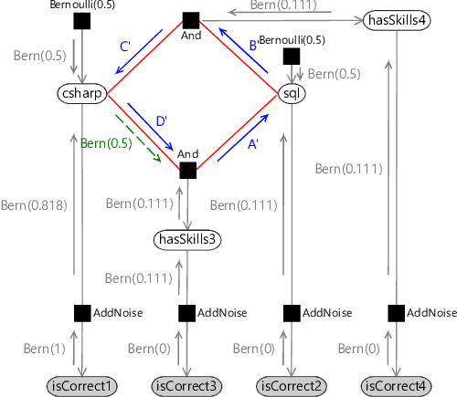
Let’s now apply loopy belief propagation to solve our model of Figure 2.14, assuming that the candidate also gets the fourth question wrong (so that isCorrect4 is false). We’ll start by laying out the model a bit differently to make the loop really clear – see Figure 2.15a. Now we need to pick a message-passing schedule for this model. A schedule which follows the guidelines above is:
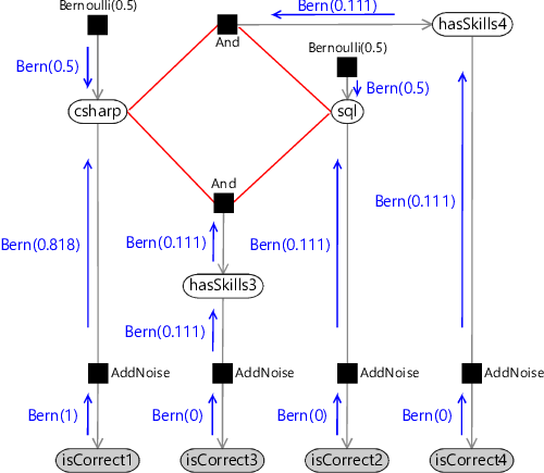
- Send messages towards the loop from the isCorrect observed nodes and the Bernoulli priors (Figure 2.15b);
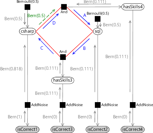
- Send messages clockwise around the loop until convergence (Figure 2.15c). We need to use one initial message to break the loop (shown in green);
- Send messages anticlockwise around the loop until convergence (Figure 2.15d). We must also use one initial message (again in green).
In fact, the messages in the clockwise and anti-clockwise loops do not affect each other since the messages in a particular direction only depend on incoming messages running in the same direction. So we can execute steps 2 and 3 of this schedule in either order (or even in parallel!).
|
Bern(1)Bern(0)Bern(0)Bern(0)Bern(0.5)Bern(0.818)Bern(0.5)Bern(0.111)Bern(0.111)Bern(0.111)Bern(0.111)Bern(0.111)
|
Bern(1)Bern(0)Bern(0)Bern(0)Bern(0.5)Bern(0.818)Bern(0.5)Bern(0.111)Bern(0.111)Bern(0.111)Bern(0.111)Bern(0.111)CDBern(0.5)BA
|
Bern(1)Bern(0)Bern(0)Bern(0)Bern(0.5)Bern(0.818)Bern(0.5)Bern(0.111)Bern(0.111)Bern(0.111)Bern(0.111)Bern(0.111)D'Bern(0.5)C'A'B'
|
For the first step of the schedule, the actual messages passed are shown in (Figure 2.15b). The messages sent around the loop clockwise are shown in Table 2.5 for first five iterations around the loop. By the fourth iteration the messages are no longer changing, which means that they have converged (and so we could have stopped after four iterations).
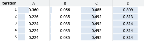
The messages for the anti-clockwise loop turn out to be identical to the corresponding messages, because the messages from hasSkills3 and hasSkills4 are the same. Given these messages, the only remaining step is to multiply together the incoming messages at csharp and sql to get the marginal distributions.
Loopy belief propagation gives the marginal distributions for csharp and sql as Bernoulli(0.809) and Bernoulli(0.010) respectively. If we use an exact inference method to compute the true posterior marginals, we get Bernoulli(0.800) and Bernoulli(0.024), showing that our approximate answers are reasonably close to the exact solution. For the purposes of this application, we are interested in whether a candidate has a skill or not but can tolerate the predicted probability being off by a percentage point or two, if it can make the system run quickly. This illustrates why approximate inference methods can be so useful when tackling large-scale inference problems. However, it is always worth investigating what inaccuracies are being introduced by using an approximate inference method. Later on, in section 2.5, we’ll look at one possible way of doing this.
Another reason for using approximate inference methods is that they let us do inference in much more complex models than is possible using exact inference. The accuracy gain achieved by using a better model, that more precisely represents the data, usually far exceeds the accuracy loss caused by doing approximate inference. Or as the mathematician John Tukey put it,
“Far better an approximate answer to the right question… than an exact answer to the wrong one.”
loopA loop is a path through a graph starting and ending at the same node which does not go over any edge more than once. For example, see the loop highlighted in red in Figure 2.15a.
treeA graph which does not contain any loops, such as the factor graphs of Figure 2.4 and Figure 2.5. When a graph is a tree, belief propagation can be used to give exact marginal distributions.
loopy graphA graph which contains at least one loop. For example, the graph of Figure 2.14 contains a loop, which may be seen more clearly when it is laid out as shown in Figure 2.15a. Loopy graphs present greater difficulties when performing inference calculations – for example, belief propagation no longer gives exact marginal distributions.
exact inferencean inference calculation which exactly computes the desired posterior marginal distribution or distributions. Exact inference is usually only possible for relatively small models or for models which have a particular structure, such as a tree. See also Panel 2.2.
approximate inferencean inference calculation which aims to closely approximate the desired posterior marginal distribution, used when exact inference will take too long or is not possible. For most useful models, exact inference is not possible or would be very slow, so some kind of approximate inference method will be needed.
loopy belief propagationan approximate inference algorithm which applies the belief propagation algorithm to a loopy graph by initialising messages in loops and then iterating repeatedly. The loopy belief propagation algorithm is defined in Algorithm 2.2.
convergedThe state of an iterative algorithm when further iterations do not lead to any change. When an iterative algorithm has converged, there is no point in performing further iterations and so the algorithm can be stopped. Some convergence criteria must be used to determine whether the algorithm has converged – these usually allow for small changes (for example, in messages) to account for numerical inaccuracies or to stop the algorithm when it has approximately converged, to save on computation.
message-passing scheduleThe order in which messages are calculated and passed in a message passing algorithm. The result of the message passing algorithm can change dramatically depending on the order in which messages are passed and so it is important to use an appropriate schedule. Often, a schedule will be iterative – in other words, it will consist of an ordering of messages to be computed repeatedly until the algorithm converges.
The following exercises will help embed the concepts you have learned in this section. It may help to refer back to the text or to the concept summary below.
- Draw a factor graph for a six-question test which assesses three skills. Identify all the loops in your network. If there are no loops, add more questions until there are.
- For your six-question test, design a message-passing schedule which uses as few initial messages as possible (one per loop). Remember that a message cannot be sent from a node unless messages have been received on all edges connected to that node (except for observed variable nodes).
- Extend your three question Infer.NET model from the previous self assessment, to include the fourth question of Figure 2.14. Use the TraceMessages attribute to see what messages Infer.NET is sending and confirm that they match the schedule and values shown in Table 2.5. If you get stuck, you can refer to the source code for this chapter [Diethe et al., 2019].
[Lauritzen and Spiegelhalter, 1988] Lauritzen, S. L. and Spiegelhalter, D. J. (1988). Local Computations with Probabilities on Graphical Structures and Their Application to Expert Systems. Journal of the Royal Statistical Society, Series B, 50(2):157–224.
[Pearl, 1988] Pearl, J. (1988). Probabilistic Reasoning in Intelligent Systems. Morgan Kaufmann, San Francisco.
[Suermondt and Cooper, 1990] Suermondt, H. and Cooper, G. F. (1990). Probabilistic inference in multiply connected belief networks using loop cutsets. International Journal of Approximate Reasoning, 4(4):283 – 306.
[Frey and MacKay, 1998] Frey, B. and MacKay, D. (1998). A revolution: Belief propagation in graphs with cycles. In In Neural Information Processing Systems, pages 479–485. MIT Press.
[Minka et al., 2014] Minka, T., Winn, J., Guiver, J., Webster, S., Zaykov, Y., Yangel, B., Spengler, A., and Bronskill, J. (2014). Infer.NET 2.6. Microsoft Research Cambridge. http://research.microsoft.com/infernet.
[Diethe et al., 2019] Diethe, T., Guiver, J., Zaykov, Y., Kats, D., Novikov, A., and Winn, J. (2019). Model-Based Machine Learning book, accompanying source code. https://github.com/dotnet/mbmlbook.