2.1 A model is a set of assumptions

When designing a model of some data, we must make assumptions about the process that gave rise to the data. In fact, we can say that the model is the set of assumptions and the set of assumptions is the model. The relationship between a model and the assumptions that it represents is so important that it is worth emphasising:

Selecting which assumptions to include in your model is a crucial part of model design. Incorrect assumptions will lead to models that give inaccurate predictions, due to these faulty assumptions. However, it is impossible to build a model without making at least some assumptions.

As you have seen in Chapter 1, in this book we will use factor graphs to represent our models. As you progress through the book, you will learn how to construct the factor graph that encodes a chosen set of assumptions. Similarly, you will learn to look at a factor graph and work out which assumptions it represents. You can think of a factor graph as being a precise mathematical representation of a set of assumptions. For example, in Chapter 1 we built up a factor graph that represented a precise set of assumptions about a murder mystery. For this application, we need to make assumptions about the process of a candidate answering some test questions if they have a particular skill set. This will define the relationship between a candidate’s underlying skills and their test answers, which we can then invert to infer their skills from the test answers.

When designing a factor graph, we start by choosing which variables we want to have in the graph. At the very least, the graph must contain variables representing the data we actually have (whether the candidate got each question right) and any variables that we want to learn about (the skills). As we shall see, it is often useful to introduce other, intermediate, variables. Having chosen the variables, we can start adding factors to our graph to encode how these variables affect each other in the question-answering process. It is usually helpful to start with the variables we want to learn about (the skills) and work through the process to finish with the variables that we can actually measure (whether the candidate got the questions right).

So, starting with the skill variables, here is our first assumption:

1. A candidate has either mastered each skill or not.

Assumptions0 2.1 means that we can represent a candidate’s skill as a binary (true/false) variable, which is true if the candidate has mastered the skill and false if they haven’t. Variables which can take one of a fixed set of values (like all the variables we have seen so far) are called discrete variables. Later in the chapter, we will encounter continuous variables which can take any value in a continuous range of values, such as any real number between 0 and 1. As we shall see, continuous variables are useful for learning the probability of events, amongst many other uses.

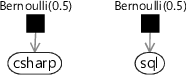
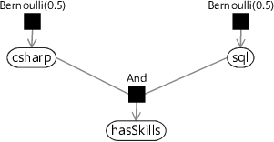
Assumptions0 2.2 means that the prior probability for each skill variable should be set neutrally to 50%, which is Bernoulli(0.5). To keep our factor graph small, we will start by considering a single candidate answering the three questions of Figure 2.1.

The above two assumptions, applied to the csharp and sql skills needed for these questions, give the following minimal factor graph:

bool variable Whether the person has the C# skill or not. csharp bool variable Whether the person has the SQL skill or not. sqlBernoulli(0.5)Bernoulli(0.5)

Figure 2.2Factor graph showing priors for the binary skill variables csharp and sql.

Remember that every factor graph represents a joint probability distribution over the variables in the graph. The joint distribution for this factor graph is:

Note that there is a term in the joint probability for every factor (black square) in the factor graph.

Continuing with the question-answering process, we must now make some assumptions about how a candidate’s test answers relate to their skills. Suppose they have all the skills for a question, we should still allow that they may get it wrong some of the time. If we gave some SQL questions to a SQL expert, how many should we expect them to get right? Probably not all of them, but perhaps they would get 90% or so correct. We could check this assumption by asking some real experts to do such a quiz and seeing what scores they get, but for now we’ll assume that getting one in ten wrong is reasonable:

3. If a candidate has all of the skills needed for a question then they will usually get the question right, except one time in ten they will make a mistake.

For questions where the candidate lacks a necessary skill, we may assume that they guess at random:

4. If a candidate doesn’t have all the skills needed for a question, they will pick an answer at random. Because this is a multiple-choice exam with five answers, there’s a one in five chance that they get the question right.

Assumptions0 2.3 and Assumptions0 2.4 tell us how to extend our factor graph to model the first two questions of Figure 2.1. We need to add in variables for each question that are true if the candidate got the question right and false if they got it wrong. Let’s call these variables isCorrect1 for the first question and isCorrect2 for the second question. Based on our assumptions, if csharp is true, we expect isCorrect1 to be true unless the candidate makes a mistake (since the first question only needs the csharp skill). Since we assume that mistakes happen only one time in ten, the probability that isCorrect1 is true in this case is 90%. If csharp is false, then we assume that the candidate will only get the question right by one time in five, which is 20%. This gives us the following conditional probability table:

Table 2.1Conditional probability table showing the probability of each value of isCorrect1 conditioned on each of the two values of csharp.

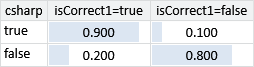
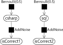
We will call the factor representing this conditional probability table AddNoise since the output is a ‘noisy’ version of the input. Because our assumptions apply equally to all skills, we can use the same factor to relate sql to isCorrect2. This gives the following factor graph for the first two questions:

bool variable Whether the person has the C# skill or not. csharp bool variable Whether the person has the SQL skill or not. sql bool variable Whether the person got question 1 correct. isCorrect1 bool variable Whether the person got question 2 correct. isCorrect2Bernoulli(0.5)Bernoulli(0.5)AddNoiseAddNoise

Figure 2.3Factor graph for the first two questions in our test.

We can write down the joint probability distribution represented by this graph by including the two new terms for the AddNoise factors:

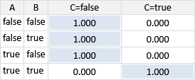
Modelling the third question is more complicated since this question requires both the csharp and sql skills. Assumptions0 2.3 and Assumptions0 2.4 refer to whether a candidate has “all the skills needed for a question”. So for question 3, we need to include a new intermediate variable to represent whether the candidate has both the csharp and sql skills. We will call this binary variable hasSkills, which we want to be true if the candidate has both skills needed for the question and false otherwise. We achieve this by putting in an And factor connecting the two skill variables to the hasSkills variable. The And factor is defined so that $\factor{And}(\var{C}|\var{A},\var{B})$ is 1 if C is equal to $\var{A} \mathrm{~AND~} \var{B}$ and 0 otherwise. In other words, it forces the child variable C to be equal to $(\var{A} \mathrm{~AND~} \var{B})$. A factor like And, where the child has a unique value given the parents, is called a deterministic factor (see Panel 2.1).

Panel 2.1Deterministic factors

When building a model, we often want to include a variable which is a fixed function of some other variables in the model. For example, we may want a binary variable to be true if all of some other binary variables are true (AND) or if any of them are true (OR). For a continuous variable, we may want it to be the sum or product of some other continuous variables.

We can achieve this by putting a deterministic factor in our factor graph. The conditional probability distribution for a deterministic factor always has a value of either 1 or 0. It is 1 if the child variable is equal to the desired function of the parent variables and 0 otherwise. For example, if we want to add a variable C which is to be equal to A AND B, we can add a deterministic factor whose conditional probability distribution is:

Notice that whenever C is equal to A AND B, the conditional probability is 1 and it is 0 elsewhere. Since the overall joint probability includes this factor as one of its terms, the probability of any configuration of variables where C is not equal to A AND B must be zero. So the deterministic factor acts as a constraint that ensures C=(A AND B) is always true.

Throughout this book you will see that deterministic factors play a vital role in a wide variety of models.

Here’s a partial factor graph showing how the And factor can be used to make the hasSkills variable that we need:

bool variable Whether the person has the C# skill or not. csharp bool variable Whether the person has the SQL skill or not. sql bool variable Whether the person has both the C# and SQL skills needed for the question. hasSkillsBernoulli(0.5)Bernoulli(0.5)And

Figure 2.4The And factor is a deterministic factor which constrains hasSkills to be true if csharp and sql are both true, and to be false in all other cases.

The joint probability distribution for this factor graph is:

The new And factor means that we now have a new And term in the joint probability distribution.

Now we can put everything together to build a factor graph for all three questions. We just need to connect hasSkills to our isCorrect3 variable, once again using an AddNoise factor:

bool variable Whether the person has the C# skill or not. csharp bool variable Whether the person has the SQL skill or not. sql bool variable Whether the person got question 1 correct. isCorrect1 bool variable Whether the person got question 2 correct. isCorrect2 bool variable Whether the person has both the C# and SQL skills needed for question 3. hasSkills bool variable Whether the person got question 3 correct. isCorrect3Bernoulli(0.5)Bernoulli(0.5)AddNoiseAddNoiseAndAddNoise

Figure 2.5Factor graph for the three multiple choice questions of Figure 2.1.

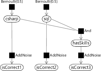
The joint probability distribution for this factor graph is quite long because we now have a total of six factor nodes, meaning that it contains six terms:

Because joint probability distributions like this one are big and awkward to work with, it is usually easier to use factor graphs as a more readable and manageable way to express a model.

It is essential that any model contains variables corresponding to the observed data, and that these variables are of the same type. This allows the data to be attached to the model by fixing these variables to the corresponding observed data values. An inference calculation can then be used to find the marginal distributions for any other (unobserved) variable in the model. For our model, we need to ensure that we can attach our test results data to the model, which consists of a yes/no result for each question depending on whether the candidate got that question right. We can indeed attach this data to our model, because we have binary variables (isCorrect1, isCorrect2, isCorrect3) which we can set to be true if the candidate got the question right and false otherwise.

There is one more assumption being made in this model that has not yet been mentioned. In fact, it is normally one of the biggest assumptions made by any model! It is the assumed scope of the model: that is, the assumption that only the variables included in the model are relevant. For example, our model makes no mention of the mental state of the candidate (tired, stressed), or of the conditions in which they were performing the test, or whether it is possible that cheating was taking place, or whether the candidate even understands the language the questions are written in. By excluding these variables from our model, we have made the strong assumption that they are independent from (do not affect) the candidate’s answers.

Poor assumptions about scope often lead to unsatisfactory results of the inference process, such as reduced accuracy in making predictions. The scope of a model is an assumption that should be critically assessed during the model design process, if only to identify aspects of the problem that are being ignored. So to be explicit, the last assumption for our learning skills model is:

5. Whether the candidate gets a question right depends only on what skills that candidate has and not on anything else.

We will not explicitly call out this assumption in future models, but it is good practice to consider carefully what variables are being ignored, whenever you are designing or using a model.

Questioning our assumptions

Having constructed the factor graph, let us pause for a moment and review the assumptions we have made so far. They are all shown together in Table 2.2.

It is very important to review all modelling assumptions carefully to ensure that they are reasonable. For example, Assumptions0 2.1 is a simplifying assumption which reduces the degree of skill that a candidate has into a simple yes/no variable. It is usual to have to make such simplifying assumptions, which are not exactly incorrect but which make the model less precise. Simplifying assumptions can be made as long as you keep in mind that these may reduce the accuracy of the results. Assumptions0 2.2 seems apparently safe since it is just assuming ignorance. However, it is also assuming that each of the skill variables are independent, that is, knowing that someone has one particular skill doesn’t tell you anything about whether they have any of the other skills. If some of the skills are related in some way, this may well not be the case. To keep the model simple, we will work with this assumption for now, but bear it in mind as a candidate for refinement later on. Assumptions0 2.3 and Assumptions0 2.4 are more subtle: is it really true that if the candidate has, say, two out of three skills needed for a question, then they are reduced to guesswork? We will continue to use these assumptions for now – later in the chapter we will show how to diagnose whether our model assumptions are causing problems and see how to revise them. Assumptions0 2.5, that no other variables are relevant, is reasonable assuming that there is a conscientious examiner administering the test. A good examiner will make sure that a candidate’s answers genuinely reflect their skills and are not affected by external conditions or cheating.

Having reviewed our assumptions by eye, we can now try the model out to ensure that the assumptions continue to make sense when applied to realistic example data.