3.1 Modelling the outcome of games

Our goal is to build a system which can assess the skills of players in online gaming. As a first step towards this, we need to look at the simpler problem of predicting the outcome of a game where we already know the skills of the players involved. This will allow us to develop many of the concepts required to solve the more complex problem of determining skills.

Suppose that Jill is going to play a game of Halo against Fred on Xbox Live. In Chapter 2 we represented a person’s software development skills by using a binary variable for each skill, indicating whether the person possessed that particular skill or not. This approach is insufficient when we consider a person’s skill at a typical Xbox game such as Halo, since there is a wide spectrum of possible skill levels. Instead, it is more appropriate to represent a person’s skill using a continuous value. The first of our modelling assumptions is therefore:

1. Each player has a skill value, represented by a continuous variable.

The stronger player is not always the winner.

We denote the skill of Jill by Jskill and the skill of Fred by Fskill. Let us suppose that Fred has a skill level of Fskill = 12.5 while Jill has a skill of Jskill = 15. These numbers appear to be completely arbitrary, and the scale on which we measure skill is indeed arbitrary. What matters, however, is how the skill values compare between players, and we shall see in a moment how to give meaning to such numbers. We have given Jill a higher skill value to indicate that she is the stronger player.

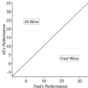
Now we run into the first of our challenges, which is that the stronger player in a game such as Halo is not always the winner. If Jill and Fred were to play lots of games against each other we would expect Jill to win more than half of them, but not necessarily to win them all. We can capture this variability in the outcome of a game by introducing the notion of a performance for each player, which expresses how well they played on a particular game. The player with the higher performance for a specific game will be the winner of that game. A player with a high skill level will tend to have a high performance, but their actual performance will vary from one game to another. As with skill, the performance is most naturally expressed using a continuous quantity. We denote Jill’s performance by Jperf and Fred’s performance by Fperf. Figure 3.2 shows Jperf plotted against Fperf. For points lying in the region above the diagonal line Jill is the winner, while below the diagonal line Fred is the winner.

Figure 3.2Schematic illustration of the values of Jill’s performance and Fred’s performance showing the areas in which Jill would be the winner and in which Fred would be the winner.

Modelling how well someone plays

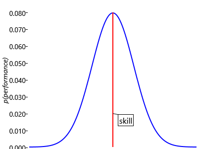
We can think of a person’s skill as their average performance across many games. For example, Jill’s skill level of 15 means her performance will have an average value of 15, but on a particular game it might be higher or lower. Once again we have to deal with uncertainty, and we shall do this using a suitable probability distribution. We anticipate that larger departures of performance from the average will be less common, and therefore have lower probability, than values which are close to the average. Intuitively the performance should therefore take the form of a ‘bell curve’ as illustrated in Figure 3.3 in which the probability of a given performance value falls off on either side of the skill value.

Figure 3.3Illustration of a ‘bell curve’ showing how the performance of a player can vary randomly around their skill value.

Because performance is a continuous quantity, this bell curve is an example of a probability density, which we encountered previously in Panel 2.4. Although we have sketched the general shape of the bell curve, to make further progress we need to define a specific form for this curve. There are many possible choices, but there is one which stands out as special in having some very useful mathematical properties. It is called the Gaussian probability density and is the density function for the Gaussian distribution.

In fact, the Gaussian distribution has so many nice properties that it is one of the most widely used distributions in the fields of machine learning and statistics. A particular Gaussian distribution is completely characterized by just two numbers: the mean, which sets the position of the centre of the curve, and the standard deviation, which determines how wide the curve is (see Panel 3.1 for discussion of these concepts). Figure 3.4 shows a Gaussian distribution, illustrating the interpretation of the mean and the standard deviation.

Figure 3.4Plot of the Gaussian distribution having mean of 15 and standard deviation of 5, showing the mean (red line) and the values which differ from the mean by plus-or-minus one standard deviation (green lines). There is roughly a 68.2% probability of a random variable with this distribution having a value lying within one standard deviation of the mean (i.e. between the two green lines), a 95.4% probability of the value lying within two standard deviations of the mean (i.e. between 5 and 25), and a 99.7% probability of the value lying within three standard deviations of the mean (i.e. between 0 and 30).

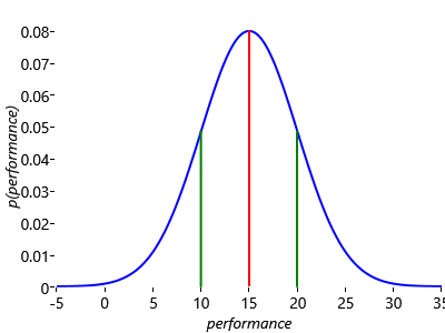
To understand the scale of the values on the vertical axis of Figure 3.4, remember that the total area under a probability distribution curve must be one. Note that the distribution is symmetrical about its maximum point – because there is equal probability of being on either side of this point, the performance at this central point is also the mean performance.

In standard notation, we write the mean as $\mu$ and the standard deviation as $\sigma$. Using this notation the Gaussian density function can be written as

The left hand side says that Gaussian$(x ; \mu, \sigma^2)$ is a probability distribution over $x$ whose value is dependent on the values of $\mu$ and $\sigma$. It is often convenient to work with the square of the standard deviation, which we call the variance and which we denote by $\sigma^2$ (see Panel 3.1). We shall also sometimes use the inverse of the variance $\tau = 1/\sigma^2$ which is known as the precision. For the most part we shall use standard deviation since this lives on the same scale (i.e. has the same units) as $x$.

Sometimes when we are using a Gaussian distribution it will be clear which variable the distribution applies to. In such cases, we can simplify the notation and instead of writing Gaussian$(x ; \mu, \sigma^2)$ we simply write Gaussian$(\mu, \sigma^2)$. It is important to appreciate that is simply a shorthand notation and does not represent a distribution over $\mu$ and $\sigma^2$.

Now let’s see how we can apply the Gaussian distribution to model a single game of Halo between Jill and Fred. Figure 3.5 shows the Gaussian distributions which describe the probabilities of various performances being achieved by Jill and Fred in their Halo game.

Excel

CSV

Figure 3.5Plot of the Gaussian distributions of performance for Jill (blue) and Fred (red).

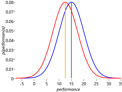
Here we have chosen the standard deviations of the two Gaussians to be the same, with $\var{perfSD} = 5$ (where ’perfSD’ denotes the standard deviation of the performance distribution). We shall discuss the significance of this choice shortly. The first question we can ask is: “what is the probability that Jill will be the winner?”. Note that there is considerable overlap between the two distributions, which implies that there is a significant chance that the performance value for Fred would be higher than that for Jill and hence that he will win the game, even though Jill has a higher skill. You can also see that if the curves were more separated (for example, if Jill had a skill of 30), then the chance of Fred winning would be much reduced.

We have introduced two further assumptions into our model, and it is worth making these explicit:

2. Each player has a performance value for each game, which is independent from game to game and has an average value is equal to the skill of that player. The variation in performance, which is the same for all players, is symmetrically distributed around the mean value and is more likely to be close to the mean than to be far from the mean.
3. The player with the highest performance value wins the game.

As written, assumption Assumptions0 3.2 expresses the qualitative knowledge that a domain expert in online games might possess, and corresponds to a bell-shaped performance distribution. This needs to be refined into a specific mathematical form and for this we choose the Gaussian, although we might anticipate that other bell-shaped distributions would give qualitatively similar results.

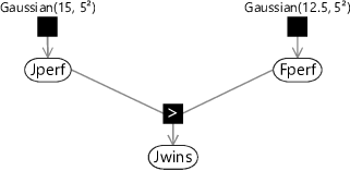
This is a good moment to introduce our first factor graph for this chapter. To construct this graph we start with the variable nodes for each random variable in our problem. So far we have two variables: the performance of Fred, which we denote by the continuous variable Fperf, and the performance for Jill, denoted by Jperf. Each of these is described by a Gaussian distribution whose mean is the skill of the corresponding player, and with a common standard deviation of 5, and therefore a variance of $5^2$:

Note that, as in section 2.6, we are using a lower-case $p$ to denote a probability density for a continuous variable, and will use an upper-case $P$ to denote the probability distribution for a discrete variable.

The other uncertain quantity is the winner of the game. For this we can use a binary variable JillWins which takes the value true if Jill is the winner and the value false if Fred is the winner. The value of this variable is determined by which of the two variables Jperf and Fperf is larger – it will be true is Jperf is larger or otherwise false. Using T for true and F for false as before, we can express this distribution by

Since probabilities sum to one, we then have

We shall refer to the conditional probability in equation (3.6) as the GreaterThan factor, which we shall denote by ‘>’ when drawing factor graphs. Note that this is a deterministic factor since the value of the child variable is fixed if the values of both parent variables are known. Using this factor, we are now ready to draw the factor graph. This has three variable nodes, each with a corresponding factor node, and is shown in Figure 3.6.

double variable Jill's performance Jperf double variable Fred's performance Fperf bool variable Whether Jill won the game JwinsGaussian(15, 5²)Gaussian(12.5, 5²)>

Figure 3.6Factor graph for a game between two players, Fred and Jill, with known skills.

Computing the probability of winning

We asked for the probability that Jill would win this game of Halo. We can find an approximate answer to this question by using ancestral sampling – refer back to section 2.5 for a reminder of what this is. To apply ancestral sampling in our factor graph we must first sample from the parent variables Jperf and Fperf and then compute the value of the child variable Jwins.

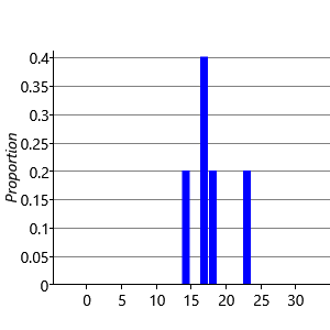
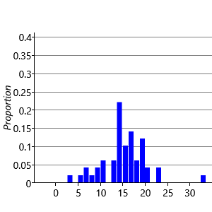
Consider first the sampling of the performance Jperf for Jill. There are standard numerical techniques for generating random numbers having a Gaussian distribution of specified mean and variance. If we generate five samples from $\dist{Gaussian}(x;15, 5^2)$ and plot them as a histogram we obtain the result shown in Figure 3.7a. Note that we have divided the height of each bar in the histogram by the total number of samples (in this case 5) and set the width of the histogram bins to be one. This ensures that the total area under the histogram is one. If we increase the number of samples to 50, as seen in Figure 3.7b, we see that the histogram roughly approximates the bell curve of a Gaussian. By increasing the number of samples we obtain a more accurate approximation, as shown in Figure 3.7c for the case of 500 samples, and in Figure 3.7d for 5,000 such samples.

(a)5 samples

(b)50 samples

(c)500 samples

(d)5,000 samples

Figure 3.7Histograms of samples drawn from the Gaussian distribution shown in Figure 3.4, with mean of 15 and standard deviation of 5.

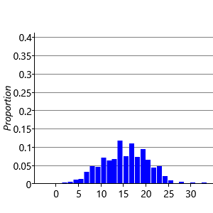
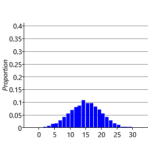
We see that we need to draw a relatively large number of samples in order to obtain a good approximation to the Gaussian. When using ancestral sampling we therefore need to use a lot of samples in order to obtain reasonably accurate results. This makes ancestral sampling computationally very inefficient, although it is a straightforward technique which provides a useful way to help understand a model or generate synthetic datasets.

Having seen how to sample from a single Gaussian distribution we can now consider ancestral sampling from the complete graph in Figure 3.6 representing a single game of Halo between Jill and Fred. We first select a performance Jperf for Jill on this specific game, corresponding to the top-level variable node on the factor graph, by drawing a value from the Gaussian distribution

Independently, we choose a performance value Fperf for Fred, which is also a top-level variable node, by drawing a sample from the Gaussian distribution

We then compute the value of the remaining variable JillWins using these sampled values. This involves comparing the two performance values, and if Jperf is greater than Fperf then JillWins is true, otherwise JillWins is false. If we repeat this sampling process many times, then the fraction of times that JillWins is true gives (approximately) the probability of Jill winning a game. The larger the number of samples over which we average, the more accurate this approximation will be. Figure 3.8 shows a scatter plot of the performances of our two players across 1,000 samples.

Figure 3.8Samples of Jill and Fred’s performances overlaid on the schematic illustration from Figure 3.2. The cloud of samples is vertically centered on Jill’s skill of 15 and horizontally centered on Fred’s skill of 12.5. The centre of the cloud is therefore above the diagonal and so more samples correspond to Jill winning than to Fred winning.

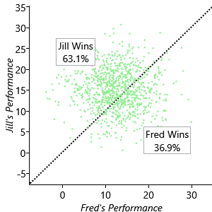
For each game we independently select the performance of each player by generating random values according to their respective Gaussian distributions. Each of these games is shown as a point on the scatter plot. Also shown is the diagonal line along which the two performances are equal. Points lying below this line represent games in which Fred is the winner, while points lying above the line are those for which Jill is the winner. We see that the majority of points lie above the line, as we expect because Jill has a higher skill value. By simply counting the number of points we find that Jill wins 63.1% of the time.

Of course this is only an approximate estimate of the probability of Jill winning. We can find the exact result mathematically by making use of the equation for the Gaussian distribution (3.1), which tells us that the probability of Jill being the winner is given by

Here CumGauss denotes the cumulative Gaussian function which is illustrated in Figure 3.9

Figure 3.9The blue curve shows a Gaussian distribution with mean of zero and a standard deviation of one. The area under this Gaussian up to the point $x$ is known as the cumulative Gaussian distribution and is shown by the red curve, as a function of $x$. For example, at $x = -1$ the area of the shaded region has the value 0.16, as indicated.

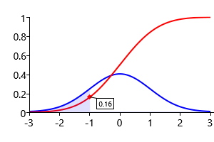
Using a numerical evaluation of this function we find that the probability of Jill winning the game is 63.8%, which is close to the value of 63.1% that we obtained by ancestral sampling.

We noted earlier that the scale on which skill is measured is essentially arbitrary. If we add a fixed number to the skills of all the players this would leave the probabilities of winning unchanged since, from equation (3.10), they depend only on the difference in skill values. Likewise, if we multiplied all the skill values by some fixed number, and at the same time we multiplied the parameter perfSD by the same number, then again the probabilities of winning would be unchanged. All that matters is the difference in skill values measured in relation to the value of perfSD.

We have now built a model which can predict the outcome of a game for two players of known skills. In the next section we will look at how to extend this model to go in the opposite direction: to predict the player skills given the outcome of one or more games.