7.3 Correcting for worker biases

We have discovered that some crowd workers are biased towards certain wrong labels for tweets with a particular true label. For example, some workers tend to give the label Neutral for tweets which should be labelled Positive or Negative. This contradicts our Assumptions0 7.4, which stated that:

4. If a worker cannot determine the true label, they will choose a label uniformly at random.

In fact, workers do not choose labels at random. They instead choose labels in a biased way that depends on the true label. If we look at the confusion matrices in Figure 7.9, then we can see each worker makes different kinds of mistakes. The confusion matrices provide a clear description of the mistakes that each worker makes. If only we could get our model to learn the confusion matrix for each worker, then it could use this to improve its accuracy. For example, for workers that incorrectly give label Neutral for tweets with true label Negative, our model could learn that when the worker provides the label Neutral then this is actually evidence for label Negative.

How can we get our model to learn a confusion matrix for each worker? First, we need to throw away all of our previous assumptions about how workers provide labels (Assumptions0 7.2 through to Assumptions0 7.5). We can then make a new assumption:

2. Each worker gives a tweet a particular label with a worker-specific probability that depends on the true label of the tweet.

Here, we are assuming that each worker has their own conditional probability table, which gives the probability of the worker assigning each label to a tweet, conditioned on the true label of the tweet. This conditional probability table has the same rows and columns as the worker’s confusion matrix and the conditional probabilities in the cells correspond to the percentage entries in the confusion matrix. In other words, the conditional probability table will represent the confusion matrix – and so learning the table for a worker will effectively mean that we are learning their personal confusion matrix.

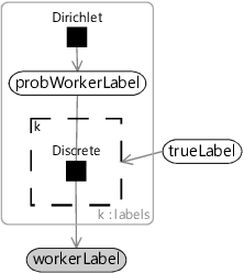
To learn the conditional probability table for a worker, we will need to represent it using random variables. Recall from section 1.1 that the probabilities in each row of a conditional probability table must add up to 1. That means each row of a conditional probability table is an array of probabilities summing to 1, just like for probLabel! So we can create a similar random variable called probWorkerLabel to contain the probabilities for a row. If we put this variable inside a plate over the labels, we will get a row per label – in other words, an entire table. To make use of this table, we need a gate for row which is turned on only when trueLabel has that value. Each gate then connects the corresponding row of the table to a Discrete factor to generate the workerLabel. The resulting factor graph is shown in Figure 7.10 – notice that it looks just like the factor graph of Figure 6.19 but with discrete/Dirichlet factors instead of Bernoulli/Beta ones.

plate of size: labels k : labels gate (on when trueLabel=Var[k]) k observed int variable The label assigned to this tweet by this worker. workerLabel int variable The true label for this tweet. trueLabel double[][] variable An array of probabilities of this worker giving a tweet each possible label, conditioned on the true label of the tweet. probWorkerLabelDirichletDiscrete

Figure 7.10A model for learning a worker’s conditional probability table. Each probWorkerLabel variable represents a row of the table. The trueLabel selects one row of the table which then provides the probabilities for choosing each possible value for the workerLabel.

In Figure 7.10 we have used a Dirichlet prior over probWorkerLabel, just like we did for probLabel. We can choose this prior for each row of the conditional probability table to encode any assumptions we want to make about the probabilities in that row. Specifically, we will assume:

3. Most workers will have a higher probability of giving the correct label than an incorrect one.

This assumption states that we expect the conditional probability of the correct label for a tweet to be higher than that for an incorrect label, for most workers. We can encode this assumption in our model by using a Dirichlet prior for each row with a higher count parameter for the correct label than for incorrect labels combined. If we choose the three incorrect labels in a row to have a count parameter of 1, then we could give the correct label a count parameter of 6, which is twice the combined counts of the three incorrect labels. These counts mean we would use Dirichlet(6,1,1,1) for the prior for the first row, Dirichlet(1,6,1,1) for the second row, Dirichlet(1,1,6,1) for the third row and Dirichlet(1,1,1,6) for the last row. These prior distributions favour having high probabilities on the diagonal entries of the CPT than on the off-diagonal entries, which is just what we want in order to satisfy Assumptions0 7.3.

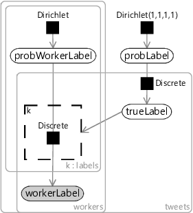
If we use the factor graph of Figure 7.10 to replace the corresponding piece of our initial model, we get the new model of Figure 7.11. This kind of model was first developed by Kim and Ghahramani. [2012] who called it the Independent Bayesian Classifier Combination (IBCC) model.

plate of size: tweets tweets plate of size: workers workers plate of size: labels k : labels gate (on when trueLabel=Var[k]) k observed int[][] variable The label assigned to this tweet by this worker. workerLabel double[] variable An array of probabilities of a tweet having each possible label. probLabel int[] variable The true label for this tweet. trueLabel double[][][] variable An array of probabilities of this worker giving a tweet each possible label, conditioned on the true label of the tweet. probWorkerLabelDirichlet(1,1,1,1)DiscreteDirichletDiscrete

Figure 7.11A biased worker model which assumes that each worker has their own biases which can be captured by a conditional probability table. The hope is that the model can learn each worker’s biases and appropriately correct for them when inferring the true label of a tweet.

We expect that the model of Figure 7.11 will be able to learn about the biases of each worker and so correct for them. The general problem of correcting for data set bias is a very important one in machine learning. Bias in data sets has been shown to lead to a form of automated discrimination, where machine learning systems have given biased outputs, for example, with respect to gender, race or economic status. A core assumption of many machine learning systems is that the training set is representative of how the system will be applied – in practice, this is often far from true. For example, face recognitions systems have often been trained on data sets with predominantly white-skinned people. Overcoming these problems to make fairer machine learning systems is a very important problem and the focus of much current work (see Holstein et al. [2019], for example). The approach we are using in this chapter shows one possible way of correcting for these kinds of biases.

Evaluating our biased worker model

We believe that our new model will be able to learn and correct for the biases of our workers and so give improved accuracy when inferring the true labels of tweets. To see if this is true, we can evaluate our new model and compare results to our initial model and to majority vote. Figure 7.12 shows the accuracy of each of our models. Looking at this figure, you can see that our new model is actually doing much worse than our initial model! In fact, its accuracy is almost down to the level of majority vote.

Excel

CSV

Figure 7.12Accuracy of our new biased worker model compared to the initial model and to majority vote. Unfortunately, our new model is less accurate than our initial model and only slightly more accurate than our majority vote baseline.

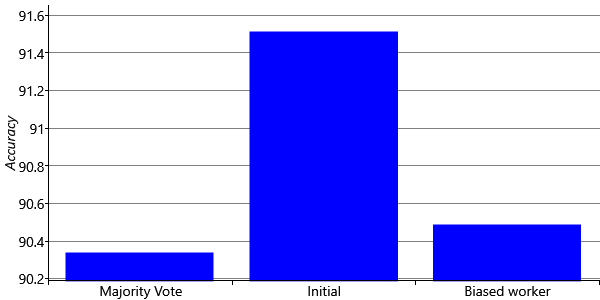
How can our new model be doing so much worse than the initial one? This is surprising because we expect our new model to be able to learn the biases of each crowd worker and so do better. This result is particularly counter-intuitive because the initial model is actually a special case of the biased worker model. We can choose a conditional probability table whose diagonal values are the ability from the previous model and zero elsewhere, and then add in a uniform distribution to each row to represent the crowd worker guessing when they do not know the true label. With these settings our new model exactly reproduces the old model. We would therefore expect that the new model would be at least as good as the old, since it could learn to fall back on the old model’s settings if necessary. Because the new model is actually doing less well, there must be some kind of problem in learning a good enough conditional probability table in probWorkerLabel. But what could this problem be?

Here, it is useful to consider what we are asking our model to learn, and from what data. For each worker, we are trying to learn a $4\times4$ conditional probability table – in other words, 16 probability values. But since each row has to add up to 1, we only really need to learn 12 of these 16 values, because one value in each row can be computed by subtracting the remaining values from 1.0. Each of these 12 values is a conditional probability of the worker giving some label for a tweet with some true label. If we were asked to estimate such a probability, we’d want to see examples of tweets with each true label and each possible worker label. For example, if we wanted to estimate the probability of a worker giving label Neutral to tweets with true label Negative, then we’d want to see lots of examples of Negative tweets so that we could estimate the proportion of these labelled as Neutral. The more examples we were given, the more accurately we’d expect to estimate the probability – so we would want lots of labels for each combination of true and worker labels. But how many do we actually have? Figure 7.13 shows how many workers provided differ amounts of labels in our training set.

Excel

CSV

Figure 7.13Histogram of the number of workers who have given different numbers of labels. The histogram shows that the majority of workers have labelled fewer than 50 tweets and many have labelled far fewer than that.

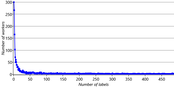
The plot shows that the majority of workers have labelled less than 50 tweets – and many have labelled far fewer. Even for workers with 50 labels, if these were split evenly amongst 12 values we are trying to learn, we would only have four or so labels per probability value – not enough to accurately estimate the probabilities. In reality the labels are not split evenly and so it is likely that we would have no data at all for many probability values. In short, we do not have enough data to learn the conditional probability tables for most of the workers. Therefore, most worker conditional probability tables will end up very uncertain – and so we will, in turn, become less certain about the true label for a tweet.

When working with data, it’s not good to be too flexible!

Another way of looking at this problem is that our model is too flexible. It allows for too many possible kinds of workers. For example, it allows for workers that always give the label Positive, for workers that always pick labels at random, for workers that deliberately give Positive for tweets that are Negative and vice versa, indeed for workers that give every possible wrong label for a each true label and with every possible probability, and so on. This is a huge number of possibilities! If we believe that workers are generally well intentioned, then many of these possibilities will likely not occur. Yet our model is requiring us rule out each unlikely possibility, and to do this for each worker individually. This task is asking too much of the available data.

Comparing more and less flexible models

A visualization of this situation is shown in Figure 7.14, which is heavily inspired by a figure from David MacKay’s excellent book [MacKay, 2003, p.344]. In this figure, the x-axis represents all possible data sets, so we can think of each point on the axis as a particular dataset, such as the marked data sets $D_A$ and $D_B$. The y-axis represents the probability of a dataset given a model, which is the model evidence (see section 6.3). The simpler model $M_1$ can only explain a limited range of possible data sets – which includes $D_A$ but excludes $D_B$. Our initial model is like this – for example, it cannot explain data sets where crowd workers have strong biases and so these will have very low probability under the model. However, because a simpler model explains fewer data sets, it can put higher probability on each one and so have higher model evidence. So for a data set like $D_A$, the simpler model $M_1$ is more probable, even though it could also be explained by the more flexible model $M_2$. The result is that predictions under $M_1$ would be more accurate than under $M_2$ – exactly the situation that we are seeing with our two models.

Figure 7.14A visualization of a simpler model $M_1$ and a more flexible model $M_2$. The x-axis represents all possible data sets and the y-axis gives the probability of each dataset under the model (the evidence). The simpler model $M_1$ can explain fewer data sets and so gives higher probability to each one than the more flexible model $M_2$. So for a data set that fits both models, like $D_A$, the simpler model is more probable. Where the additional flexibility of $M_2$ is needed to explain the data set, as is the case for $D_B$, then the more complex model becomes more probable.

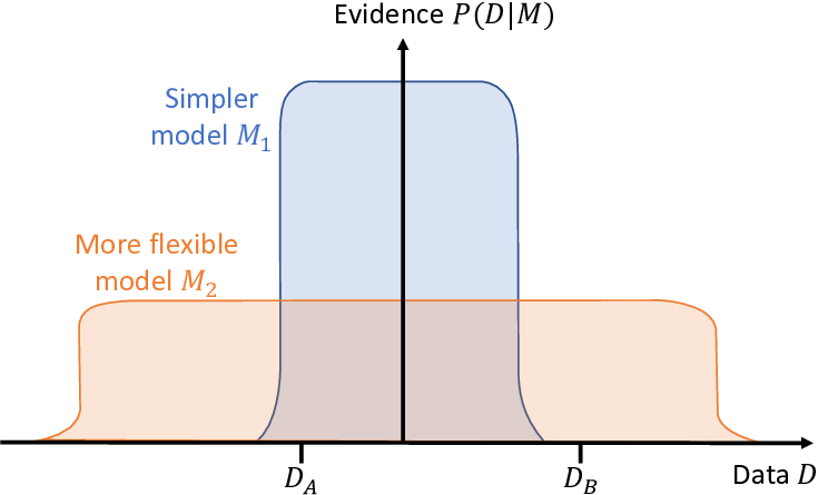
The figure also shows another data set $D_B$ which can be explained by the more flexible model $M_2$, but not by the simpler model $M_1$. Here the additional flexibility of $M_2$ is essential for explaining the data set and so will have much higher model evidence than $M_1$. In general, the more restrictive the assumptions encoded by the model, the smaller the range of data sets that will be explained well by the model. If the actual data set lies in this range then this restrictive model will work better than a model with less restrictive assumptions.

So the reason that the new model is working less well, is that it is too flexible. The model is trying to learn a conditional probability table for every single worker and there is just insufficient data to do this well. We need to find a way to learn our conditional probability tables from much more data – to learn how we can do this, read on!