4.6 Learning as emails arrive
So far we’ve been able to train our model on a large number of emails at once. But for our application we need to be able to learn from a new email as soon as a user replies to it, or as soon as it becomes clear that the user is not going to reply to it. We cannot wait until we have received a large number of emails, then train on them once and use the trained model forever. Instead, we have to keep training the model as new emails come in and always use the latest trained model to make predictions.
As we saw in section 3.3 in the previous chapter, we can use online learning to continually update our model as we receive new training data. In our model online learning is straightforward: for each batch of emails that have arrived since we last trained, we use the previous posterior distributions on weight and threshold as the priors for training. Once training on the batch is complete, the new posterior distributions over weight and threshold can be used for making predictions. Later when the next batch of emails is trained on, these posterior distributions will act as the new priors. We can check how well this procedure works by dividing our training data into batches and running online learning as each batch comes in. We can then evaluate this method in comparison to offline training, where all the training data seen up to that point is presented at once. Figure 4.20 shows the AUC and AP averaged across all 10 users using either offline training or online training with different batch sizes.
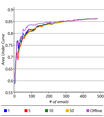
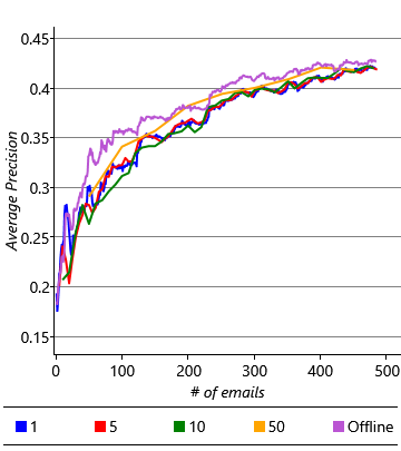
These results show that online learning gives an accuracy similar to, but slightly lower than offline training, with larger batch sizes giving generally better accuracy. The plots also show that the difference in accuracy decreases as more emails are received. So it seems like online learning could be a suitable solution, once sufficient emails have been received. But this brings us to another problem: it takes around 400 to 500 emails for the average precision to get close to a stable value. For a time before that number is reached, and particularly when relatively few emails have been trained on, the accuracy of the classifier is low. This means that the experience for new users would be poor. Of course, we could wait until the user has received and acted on sufficient emails, but for some users this could take weeks or months. It would be much better if we could give them a good experience straight away. The challenge of making good predictions for new users where there is not yet any training data is known as a cold start problem.
Modelling a community of users
We’ve already shown that we can solve certain prediction problems by changing the feature set. But in this case, there is no change to the feature set that can help us – we cannot even compute feature values until we have seen at least one email! But since we have a classification model rather than a fixed classification algorithm, we have an additional option available to us: to change the model.

Learning from many users will help us to make better predictions for a new user.
How can we change our model to solve the cold start problem? We can exploit the fact that different users tend to reply to the same kinds of emails. For example, users tend to be more likely to reply to emails where they are first on the To line or where the email is forwarded to them. This suggests that we might expect the learned weights to be similar across users, at least for those feature buckets that capture behaviours common amongst users. However, there may also be other feature buckets which capture differences in the behaviour from user to user, where we may expect the learned weights to differ between users. To investigate which feature buckets are similar across users, we can plot the learned weights for the first five of our users, for all feature buckets that they have in common (that is, all buckets except those of the Sender and Recipients features). The resulting plot is shown in Figure 4.21.
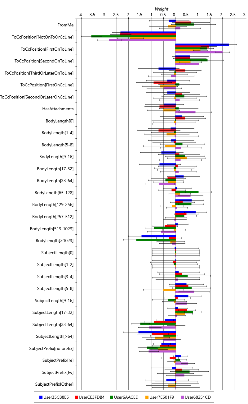
As you can see, for many feature buckets, the weights are similar for all five users and even for buckets where there is more variability across users the weights tend to be all positive or all negative. But in a few cases, such as the FromMe feature, there is more variability from user to user. This variability suggests that these features capture differences in behaviour between users, such as whether a particular user sends emails to themselves as reminders. Overall it seems like there is enough similarity between users that we could exploit this similarity to make predictions for a completely new user. To do this, we need to make a new modelling assumption about how the weights vary across multiple users:
- Across many users the variability in the weight for a feature bucket can be captured by a Gaussian distribution.
This assumptions says that we can represent how a weight varies across users by an average weight (the mean of the Gaussian distribution) and a measure of how much a typical user’s weight deviates from this average (the standard deviation of the Gaussian distribution).
Let’s change our model to add in this assumption. Since we are now modelling multiple users, we need to add a plate across users and put our entire existing model inside it. The only variables outside of this new plate will be two new variables per feature bucket: weightMean to capture the average weight across users and weightPrecision to capture the precision (inverse variance) across users. We then replace the Gaussian(0,1) factor inside the plate (that we used to use as a prior) by a Gaussian factor connected to weightMean and weightPrecision. The resulting factor graph is shown in Figure 4.22.
|
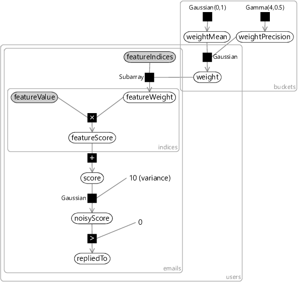
You’ll notice that we have used precision (inverse variance) rather than variance to capture the variability in weights across users. A high weightPrecision for a bucket means that its weight tends to be very similar from user to user, whilst a low weightPrecision means the bucket weight tends to vary a lot from user to user. We choose to use precision because we are now trying to learn this variability and it turns out to be much easier to do this using a precision rather than a variance. This choice allows us to use a gamma distribution to represent the uncertainty in the weightPrecision variable, either when setting its prior distribution or when inferring its posterior distribution. The gamma distribution is a distribution over continuous positive values (that is, values greater than zero). We need to use a new distribution because precisions can only be positive – we cannot use a Gaussian distribution since it allows negative values, and we cannot use a beta distribution since it only allows values between zero and one. The gamma distribution also has the advantage that it is the conjugate distribution for the precision of a Gaussian (see Panel 3.2 and Bishop [2006]).
The gamma distribution has the following density function:
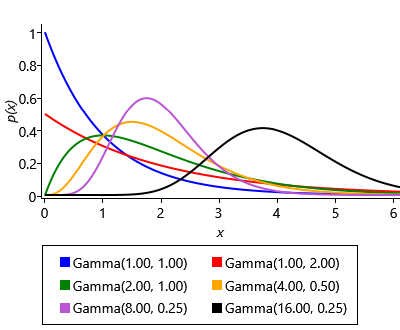
where is the gamma function, used to ensure the area under the density function is 1.0. The gamma distribution has two parameters: the shape parameter and the scale parameter – example gamma distributions with different values of these parameters are shown in Figure 4.23a. Confusingly, the gamma distribution is sometimes parameterised by the shape and the inverse of the scale, called the rate. Since both versions are common it is important to check which is being used – in this book, we will always use shape and scale parameters.
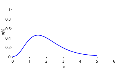
Since we have relatively few users, we will need to be careful in our choice of gamma prior for weightPrecision since it will have a lot of influence on how the model behaves. Usually we expect the precision to be higher than 1.0, since we expect most weights to be similar across users. However, we also need to allow the precision to be around 1.0 for those rarer weights that vary substantially across users. Figure 4.23b shows a Gamma(4,0.5) distribution that meets both of these requirements.
There is one more point to discuss about the model in Figure 4.22, before we try it out. If you are very observant, you will notice that the threshold variable has been fixed to zero. This is because we want to use our communal weightMean and weightPrecision to learn about how the threshold varies across users as well as how the weights vary. To do this, we can use a common trick which is to fix the threshold to zero and create a new feature which is always on for all emails – this is known as the bias. The idea is that changing the score by a fixed value for all emails is equivalent to changing the threshold by the same value. So we can use the bias feature to effectively set the threshold, whilst leaving the actual threshold fixed at 0. Since feature weights have a Gaussian(0,1) prior but the threshold has a Gaussian(0,10) prior, we need to set the value of this new bias feature to be , in order to leave the model unchanged – if we have a variable whose uncertainty is Gaussian(0,1) and we multiply it by , we get a variable whose uncertainty is Gaussian(0,10), as required.
Solving the cold start problem

A hands-on solution to the cold start problem
We can now train our communal model on the first five users (the users whose weights were plotted in Figure 4.21). Even though we have substantially changed the model, we are still able to use expectation propagation to do inference tasks like training or prediction. So we do not need to invent a new algorithm to do joint training on multiple users – we can just run the familiar EP algorithm on our extended model.
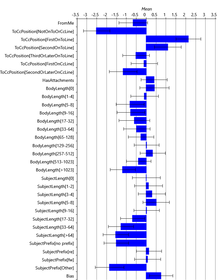
Figure 4.24 shows the community weight distributions learned: each bar shows the mean of the posterior over weightMean and the error bars show a standard deviation given by the mean value of weightPrecision. Note the different use of error bars – to show weightPrecision (the learned variability across users) rather than the uncertainty in weightMean itself. If you compare the distributions of Figure 4.24 with the individual weights of Figure 4.21, you can see how the learned distributions have nicely captured the variability in weights across users.
To apply our learned community weight distributions for a new user, we can use the same model configured for a single user with the priors over weightMean and weightPrecision replaced by the Gaussian and gamma posteriors learned from the first five users. We can use this model to make predictions even when we have not seen any emails for the new user. But we can also use the model to do online training, as we receive emails for a new user. As we do online training using the community model, we can smoothly evolve from making generic predictions that may apply to any user to making personalised predictions specific to the new user. This evolution happens entirely automatically through doing inference in our model – there is no need for us to specify an ad-hoc procedure for switching from community to personalised predictions.
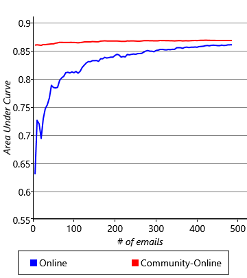
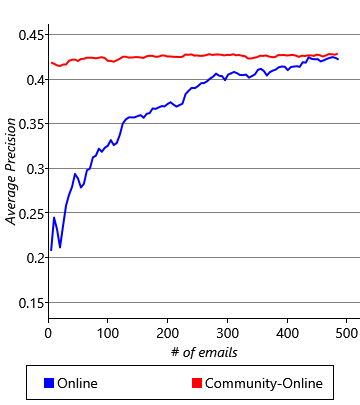
Figure 4.25 shows the accuracy of predictions made using online training in the community model compared to the individual model (using a batch size of 5) for varying amounts of training data. For this plot we again average across all ten users – we make prediction results for the first five users using a separate community model trained on the last five users. The results are very satisfactory – the initial accuracy is high (an average AP of 41.8%) and then it continues to rise smoothly until it reaches an average AP of 43.2% after 500 emails have been trained on. As we might have hoped, our community model is making good predictions from the start, which then become even better as the model personalizes to the individual user. The cold start problem is solved!
In the production system used by Exchange, we had a much larger number of users to learn community weights from. In this case, the posteriors over weightMean and weightPrecision became very narrow. When these posteriors are used as priors, the values of weightMean and weightPrecision are effectively fixed. This allows us to make a helpful simplification to our system: once we have used the multi-user model to learn community weight distributions, we can go back to the single user model to do online training and make predictions. All we need to do is replace the Gaussian(0,1) prior in the single user model with a Gaussian prior whose mean and precision are given by the expected values of the narrow weightMean and weightPrecision distributions. So, in production, the multi-user model is trained once offline on a large number of users and the learned community weight distributions are then used to do training and prediction separately for each user. This separation makes it easier to deploy, manage and debug the behaviour of the system since each user can be considered separately.
There is one final thing to do before we deploy our system to some beta testers. Remember the test sets of email data that we put to one side at the start of the chapter? Now is the time to break them out and see if we get results on the test sets that are comparable to the results we have seen on our validation sets. Comparative results for the validation and test sets are shown in Table 4.5.
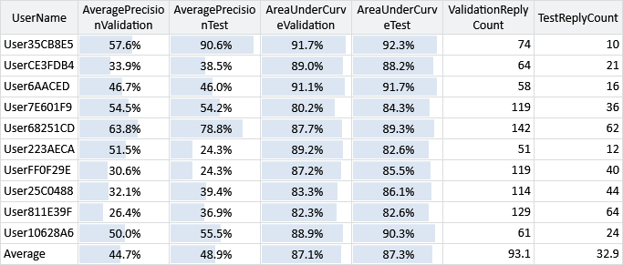
The table shows that the AUC measurements for the users’ test sets are generally quite similar to those of the validation sets, with no obvious bias favouring one or the other. This suggests that in designing our model and feature set we have not overfit to the validation data. The AP measurements are more different, particularly for some users – this is because the test sets are quite small and some contain only a few replied-to emails. In such situations, AP measurements become quite noisy and unreliable. However, even if we focus on those users with more replied to emails, it does not appear that the test AP is consistently lower than the validation AP. So both evaluation metrics suggest that there is no fundamental difference between test and validation set accuracies and so we should expect to achieve similar prediction accuracy for real users.
Final testing and changes
At this point, the prediction system was deployed to beta testers for further real-world testing. Questionnaires were used to get feedback on how well the system was working for users. This testing and feedback highlighted two additional issues:
- The predictions appeared to get less accurate over time, as the user’s behaviour evolved, for example, when they changed projects or changed teams the clutter predictions did not seem to change quickly enough to match the updated behaviour.
- The calibration of the system, although correct on average, was incorrect for individual users. The predicted probabilities were too high for some users and too low for others.
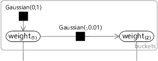
Investigation of the first issue identified a similar problem to the one we diagnosed in Chapter 3. We have assumed that the weights in the model are fixed across time for a particular user. This assumption does not allow for user behaviour to change. The solution was to change the model to allow the weights to change over time, just as we allowed the skills to change over time in the TrueSkill system. The modified model has random variables for each bucket weight for each period of time, such as a variable per week. Figure 4.26a shows an example model segment that contains weights for two consecutive weeks and . To allow the weights to change over time, the weight for the second week is allowed to vary slightly from the weight for the first week, through adding Gaussian noise with very low variance. As with the TrueSkill system, this change allows the system to track slowly-changing user behaviours.
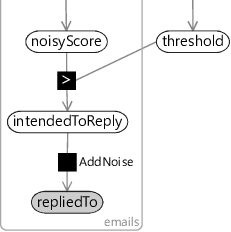
The second issue was harder to diagnose. Investigation of the issue found that the too-high predicted probabilities occurred for users that had a low volume of clutter and the too-low predicted probabilities occurred for users that had a high volume of clutter. It turned out that the problem was the noisy ground truth labels that we encountered in section 4.5 – for users with a high volume of clutter, a lot of clutter items were incorrectly labelled as not clutter and vice versa for users with a low volume of clutter. Training with these incorrect labels introduced a corresponding bias into the predicted probability of clutter. The solution here is to change the model to represent label noise explicitly. For example, for reply prediction, we can create a new variable in the model intendedToReply representing the true label of whether the user truly intended to reply to the message. We then define the observed label repliedTo to be a noisy version of this variable, using a factor like the AddNoise factor that we used back in Chapter 2. Figure 4.26b shows the relevant piece of a modified model with this change in place. Following this change, the calibration was found to be much closer to ideal across all users and the systematic calibration variation for users with high or low clutter volume disappeared.
In addressing each of these issues we needed to make changes to the model, something that would be impossible with a black box classification algorithm, but which is central to the model-based machine learning approach. With these model changes in place, the Clutter prediction system is now deployed as part of Office365, helping to remove clutter emails from peoples’ inboxes. Figure 4.27 shows a screenshot of the system in action, all using model-based machine learning!

cold start problemThe problem of making good predictions for a new entity (for example, a new user) when there is very little (or no) training data available that is specific to that entity. In general, a cold start problem can occur in any system where new entities are being introduced – for example, in a recommendation system, a cold start problem occurs when trying to predict whether someone will like a newly released movie that has not yet received any ratings.
gamma distributionA probability distribution over a positive continuous random variable whose probability density function is
where is the gamma function, used to ensure the area under the density function is 1.0. The gamma distribution has two parameters shape parameter and the scale parameter .
The plot below shows gamma distributions with different values of and :
biasA feature which is always on for all data items. Since the bias feature is always on, its weight encodes the prior probability of the label. For example, the bias weight might encode probability that a user will reply to an email, before we look at any characteristics of that particular email. Equivalently, use of a bias features allows the threshold variable to be fixed to zero, since it is no longer required to represent the prior label probability.
[Bishop, 2006] Bishop, C. M. (2006). Pattern Recognition and Machine Learning. Springer.


 Excel
Excel CSV
CSV