4.2 A model for classification

The problem of predicting a label, such as ‘reply’ or ‘not reply’, for a data item is called classification. Systems that perform classification are known as classifiers, and are probably the most widely used machine learning algorithms today. There are many different classification algorithms available and, for a particular prediction task, some will work better than others. A common approach to solving a classification problem is to try several different classification algorithms and see which one works the best. This approach ignores the underlying reason that the classification algorithms are making different predictions on the same data: that each algorithm is implicitly making different assumptions about the data. Unfortunately, these assumptions are hidden away inside each algorithm.

You may be surprised to learn that many classification algorithms can be interpreted as doing approximate inference in some probabilistic model. So rather than running a classification algorithm, we can instead build the corresponding model and use an inference algorithm to do classification. Why would we do this instead of using the classification algorithm? Because a model-based approach to classification gives us several benefits:

• The assumptions in the classifier are made explicit. This helps us to understand what the classifier is doing, which can allow us to improve how we use it to achieve better prediction accuracy.
• We can modify the model to improve its accuracy or give it new capabilities, beyond those of the original classifier.
• We can use standard inference algorithms to both train the model and to make predictions. This is particularly useful when modifying the model, since the training and prediction algorithms remain in sync with the modified model. Also, different algorithms have different trade-offs between speed and accuracy. We can choose an algorithm that best suits our needs, whilst retaining all of our modelling assumptions.

These are not small benefits – in this chapter you will see how all three will be crucial in delivering a successful system. We will show how to construct the model for a widely used classifier from scratch, by making a series of assumptions about how the label arises given a data item. We will then show how to extend this initial classification model, to achieve various capabilities needed by the email classification system. Throughout the evolution of the model we will use a standard inference algorithm (expectation propagation) for training and prediction.

Before we construct the model, we need to understand how a classifier with a fixed set of assumptions could possibly be applied to many different problems. This is possible because classifiers require the input data to be transformed into a form which matches the assumptions encoded in the classifier. This transformation is achieved using a set of features (a feature set), where a feature is a function that acts on a data item to return one or more values, which are usually binary or continuous values. In our model we will use features that return continuous values in the range 0.0 to 1.0. For example, our first feature will return 1.0 if the user is mentioned on the To line of the email or 0.0 otherwise – we’ll call this the ToLine feature. It is these feature values, rather than the data item itself, that are fed into the classifier. So, rather than changing the assumptions in the classifier, we use features to transform the data to match the assumptions already built in to the classifier.

Another important simplification that a classifier makes is that it only ever makes predictions about the label variable assuming that the corresponding values for the features are known. Because it always conditions on these known feature values, the model only needs to represent the conditional probability $P(\mathrm{label}|\mathrm{features})$ rather than the joint distribution $P(\mathrm{label},\mathrm{features})$. Because it represents a conditional probability, this kind of model is called a conditional model. It is convenient to build a conditional model because we do not need to model the data being conditioned on (the feature values) but only the probability of the label given these values. This brings us to our first modelling assumption.

1. The feature values can always be calculated, for any email.

By always, we mean always: during training, when doing prediction, for every single email ever encountered by the system. Although convenient, the assumption that the feature values can always be calculated makes it difficult to handle missing data. For example, if the sender of an email is not known, any features requiring the sender cannot be calculated. Strictly, this would mean we would be unable to make a prediction. In practice, people commonly provide a default feature value if the true value is not available, even though this is not the correct thing to do. For example in the sender case it is equivalent to treating all emails with missing senders as if they came from a particular ‘unknown’ sender. The correct thing to do would be to make a joint model of the feature values and marginalise over any missing values – but, if data is rarely missing, the simpler approach is often sufficiently good – indeed it is what we shall use here.

A one-feature classification model

We will start by building a model that uses only one feature to predict whether a user will reply to an email: whether the user is on the To line or not (the ToLine feature). Since we are building a conditional model, we only need to consider the process of generating the label (whether the user replied to the email or not) from the feature value. The variable we are trying to generate is therefore a binary label that is true if the user replied to the mail or false otherwise – we will call this variable repliedTo. This repliedTo variable is the variable that we will observe when training the model and which we will infer when making predictions.

It would be difficult to define the process of generating this binary repliedTo variable directly from the continuous feature values, since it is not itself a continuous variable. Instead, we introduce an intermediate variable that is continuous, which we shall call the score. We will assume that the score will be higher for emails which having a higher probability of reply and lower for emails which have a lower probability of reply. Here is the assumption:

2. Each email has an associated continuous score which is higher when there is a higher probability of the user replying to the email.

Notice that, unlike a probability, the continuous score value is not required to lie between zero and one but can take on any continuous value. This makes it an easier quantity to model since we do not have to worry about keeping its value constrained to be between zero and one.

We are now ready to make an assumption about how the feature value for an email affects its score.

3. If an email’s feature value changes by $x$, then its score will change by $\mathit{weight}\times x$ for some fixed, continuous weight.

This assumption says that the score for an email is either always higher if the feature value increases (if the weight is positive) or always lower if the feature value increases (if the weight is negative) or is not affected by the feature value (if the weight is zero). The size of any change in score is controlled by the size of the weight: a larger weight means a particular change in feature value produces a larger change in the score. Remember that, according to our previous assumption, a higher score means a higher reply probability and lower score means a lower reply probability.

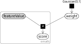
To build a factor graph to represent Assumptions0 4.3 we first need a continuous featureValue variable to hold the value of the feature for each email (so it will be inside a plate across the emails). Since this variable will always be observed, we always show it shaded in the factor graph (Figure 4.1). We also introduce a continuous weight variable for the feature weight mentioned in the assumption. Because this weight is fixed, it is the same for all emails and so lies outside the emails plate. We can then model Assumptions0 4.3 by multiplying the featureValue by the weight, using a deterministic multiplication factor and storing the result in continuous score variable. The factor graph for a single feature modelled in this way is shown in Figure 4.1.

plate of size: emails emails observed double[] variable The value of this feature, for each email. featureValue double variable The weight for this feature. weight double[] variable The score for this feature for each email, which is the feature value multipled by the weight. scoreGaussian(0,1)×

Figure 4.1Factor graph for a single feature. Each email has a featureValue which is multiplied by a single common weight to give a score for that email. A positive weight means that the score increases if the feature value increases. A negative weight means that the score decreases if the feature value increases. A higher score corresponds to a higher probability that the email is replied to.

In drawing the factor graph, we’ve had to assume some prior distribution for weight. In this case, we have assumed that the weight is drawn from a Gaussian distribution with zero mean, so that it is equally likely to be positive or negative.

4. The weight for a feature is equally likely to be positive or negative.

We have also the prior distribution to be Gaussian with variance 1.0 (so the standard deviation is also 1.0). This choice means that the weight will most often be in the range from -1.0 to 1.0, occasionally be outside this in the range -2.0 to 2.0 and very occasionally be outside even that range (as we saw in Figure 3.4). We could equally have chosen any value for the variance, which would have led to different ranges of weight values so there is no implied assumption here. The effect of this choice will depend on the feature values which multiply the weight to give the score and also on how we use the score, which we will look at next.

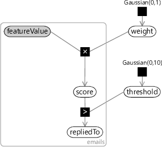
We now have a continuous score variable which is higher for emails that are more likely to be replied to and lower for emails that are less likely to be replied to. Next we need to convert the score into a binary repliedTo variable. A simple way to do this is to threshold the score – if it is above some threshold then repliedTo is true, otherwise false. We can do this by adding a continuous threshold variable and use the deterministic GreaterThan factor that we met in the previous chapter:

plate of size: emails emails observed double[] variable The value of this feature. featureValue double variable The weight for this feature. weight double variable The threshold score for replying. threshold double[] variable The score for this feature, which is the product of the feature value and the weight. score bool[] variable Whether the message is replied to. repliedToGaussian(0,1)Gaussian(0,10)×>

Figure 4.2Factor graph of Figure 4.1 extended so that if the score is greater than a threshold the binary repliedTo variable is true, otherwise it is false.

Here we’ve chosen a $\dist{Gaussian}(0,10)$ prior for the threshold – we’ll discuss this choice of prior shortly. Now suppose we try to train this one-feature model on the training set for one of our users. We can train the model using probabilistic inference as usual. First we fix the value of repliedTo for each email (by seeing if the user actually did reply to the email)and also the ToLine featureValue – which is always available since we can calculate it from the email To line. Given these two observed values for each email, we can train by inferring the posterior distributions for weight and threshold.

Unfortunately, if we attempt to run inference on this model then any inference algorithm we try will fail. This is because some of the observed values have zero probability under the model. In other words, there is no way that the data-generating process encoded by our model could have generated the observed data values. When your data has zero probability under your model, it is a sure sign that the model is wrong!

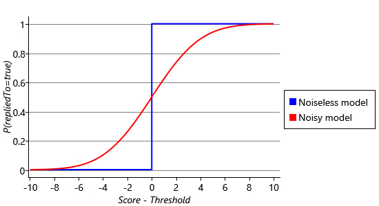
The issue is that the model is wildly overconfident. For any weight and threshold values, it will always predict repliedTo to be true with 100% certainty if the score is greater than the threshold and predict repliedTo to be false with 100% certainty otherwise. If we plot the reply probability against the score, it abruptly moves from 0% to 100% as the score passes the threshold (see the blue line in Figure 4.3). We will only be successful in training such a model if we are able to find some weight and threshold that perfectly classifies the training set – in other words gives a score above the threshold for all replied-to training emails and a score below the threshold for all emails that were not replied to. As an example, this would be possible if the user replied to every single email where they were on the To line and did not reply to every single other email. If there is even a single email where this is not the case, then its observed label will have zero probability under the model. For example, suppose a not-replied-to email has a score above the threshold – the prediction will be that repliedTo is true with probability 1.0 and so has zero probability of being false. But in this case repliedTo is observed to be false, which has zero probability and is therefore impossible under the model.

Excel

CSV

Figure 4.3Plot of the predicted probability of reply as the score varies relative to the threshold for the noiseless model of Figure 4.2 and a noisy score model which adds Gaussian noise to the score before thresholding it. For the noiseless model, the reply probability abruptly changes from 0.0 to 1.0 as the score passes the threshold. In contrast, for the noisy model, the reply probability varies smoothly from near 0.0 to near 1.0 over a range of score values (from about -8 to +8).

Looking back, Assumptions0 4.2 said that the reply probability would always be higher for emails with a higher score. But in fact, in our current model, this assumption does not hold – if we have two positive scores one higher than the other, they will both have the same 100% probability of reply. So our model is instead encoding the assumption that the reply probability abruptly changes from 0 to 100% as the score increases – it is this overly strong assumption that is causing training to fail.

Adding noise to a model can be helpful when it does not perfectly represent the data.

To better represent Assumptions0 4.2, we need the reply probability to increase smoothly as the score increases. The red curve in Figure 4.3 shows a much smoother relationship between the score and the reply probability. This curve may look familiar to you, it is the cumulative density function for a Gaussian distribution, like the ones that we saw in Figure 3.9 in the previous chapter. We’d like to change our model to use this smooth curve. We can achieve this by adding a Gaussian-distributed random value to the score before we threshold it. These are called ‘noise’ values, because they take the clean 0% or 100% prediction and make it ‘noisy’. Now, even if the score is below the threshold, there is a small probability that the noisy version will be above the threshold (and vice versa) so that the model can tolerate misclassified training examples. The exact probability that this will happen will depend on how far the score is below the threshold and the probability that the added Gaussian noise will push it above the threshold. This probability is given by the cumulative density function for the Gaussian noise, and so you end up with the curve shown in Figure 4.3.

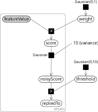
Since the predicted probability varies smoothly from 0.0 to 1.0 over a range of score values, the model can now vary the confidence of its predictions, rather than always predicting 0% or 100%. The range of values that this happens over (the steepness of the curve) is determined by the variance of the Gaussian noise. The plot in Figure 4.3 is for a noise variance of 10, which is the value that we will use in our model, for reasons we will discuss in a moment. So let’s add a new continuous variable called noisyScore and give it a Gaussian distribution whose mean is at score and whose variance is 10. This gives the factor graph of Figure 4.4.

plate of size: emails emails observed double[] variable The value of this feature. featureValue double variable The weight for this feature. weight double variable The threshold score for replying. threshold double[] variable The score for this feature, which is the product of the feature value and the weight. score double[] variable Score with added Gaussian noise. noisyScore double variable 10 (variance) bool[] variable Whether the message is replied to. repliedToGaussian(0,1)Gaussian(0,10)×Gaussian>

Figure 4.4Factor graph of a classification model with one feature. The model uses a Gaussian factor to introduce uncertainty in the prediction of repliedTo for a particular score.

In choosing a variance of 10, we have set how much the score needs to change in order to change the predicted probability. Remember that our weights are normally in the range -1.0 to 1.0, sometimes in the range -2.0 to 2.0 and occasionally outside this range. Looking at Figure 4.3 you can see that to change the predicted probability from a ‘don’t know’ prediction of 50% to a confident prediction of, say, 85% means that the score needs to change by about 3.0. If we choose feature values in the range -1.0 to 1.0 (which we will), this means that we are making the following assumption:

5. A single feature normally has a small effect on the reply probability, sometimes has an intermediate effect and occasionally has a large effect.

This assumption prevents our classification model from becoming too confident in its predictions too quickly. For example, suppose the system sees a few emails with a particular feature value, say ToLine=1.0, which are then all replied to. How confident should the system be at predicting reply for the next email with ToLine=1.0? The choice of noise variance encodes our assumption of this confidence. Setting the noise variance to a high value means that the system would need to see a lot of emails to learn a large weight for a feature and so would make underconfident predictions. Setting the noise variance too low would have the opposite effect and the system would make confident predictions after only a few training emails. A variance of 10 is a suitable intermediate value that avoids making either under- or over-confident predictions.

We can now try training this new model on the emails of one of our users, say, User35CB8E5. As in Chapter 3, we can use expectation propagation to perform inference. This gives Gaussian distributions over weight and threshold of Gaussian(3.77,0.028) and Gaussian(7.63,0.019) respectively.

We can now use these Gaussian distributions to make predictions on a new email (or several emails), using online learning, as we saw in Chapter 3. To do this, we replace the priors over weight and threshold with the learned posterior distributions. Then we fix the feature values for each email and run inference to compute the marginal distribution over repliedTo. Since we’ve only got one feature in our model and it only has two possible values, the model can only make two possible predictions for the reply probability, one for each feature value. Given the above Gaussian distributions for the weight and threshold, the predicted probability of reply for the two values of the ToLine feature are shown in Table 4.2a. As we might have expected, the predicted probability of reply is higher when the user is on the To line (ToLine=1.0) than when the user is not on the To line (ToLine=0.0).

To check whether these predicted probabilities are reasonable, we can compute the actual fraction of emails with each feature value that were replied to in the training set. The predicted probabilities should be close to these fractions. The counts of replied-to and not-replied-to emails with each feature value are shown in Table 4.2b, along with the fraction replied to computed from these counts.

Excel

CSV

(a)

Excel

CSV

(b)

Table 4.2(a) Predicted probability of reply for our one-feature model, for each feature value. (b) For each feature value: the number of emails that were replied to, the number of emails that were not replied to and the fraction of emails that were replied to for the emails of User35CB8E5. Reassuringly, these fractions are close to the predicted probabilities of the learned model.

These computed fractions are very close to the predicted probabilities, which gives us some reassurance that we have learned correctly from our data set. Effectively, we have provided a long-winded way of learning the conditional probability table given in Table 4.2a! However, if we want to use multiple features in our model, then we cannot use a conditional probability table, since it would become unmanageably large as the number of features increased. Instead, we will use the score variables to provide a different, scalable approach for combining features, as we will see in the next section.