-

Want a paper copy?
You can now buy the book!
All royalties go to the Cystic Fibrosis Trust.Spotted an error? Have comments?
Let us know!Get hands on with source code for the book.
4.4 Designing a feature set
To use our classification model, we need to design features to transform the data to conform as closely as possible to the assumptions built into the model (Table 4.3). For example, to satisfy Assumptions0 4.7 (that features contain all relevant information about the user’s actions) we need to make sure that our feature set includes all features relevant to predicting reply. Since pretty much any part of an email may help with making such a prediction, this means that we will have to encode almost all aspects of the email in our features. This will include who sent the email, the recipients of the email on the To and Cc lines, the subject of the email and the main body of the email, along with information about the conversation the email belongs to.
When designing a new feature, we need to ensure that:
- the feature picks up on some informative aspect of the data,
- the feature output is of the right form to feed into the model,
- the feature provides new information about the label over and above that provided by existing features.
In this section, we will show how to design several new features for our feature set, while ensuring that they meet the first two of these criteria. In the next section we will show how to check the third criterion by evaluating the system with and without certain features.
Features with many states
So far, we have represented where the user appears on the email using a ToLine feature. This feature has only two states: the user is either on the To line or not. So the feature ignores whether the user is on the Cc line, even though we might expect a user to be more likely to reply to an email if they appear on the Cc line than if they do not appear at all. The feature also ignores the position of the user on the To/Cc line. If the user is first on the To line we might expect them to be more likely to reply than if they are at the end of a long list of recipients. We can check these intuitions using our data set by finding the actual fraction of all training/validation emails that were replied to in a number of cases: when the user is first, second or later than second on the To line, when the user is first or elsewhere on the Cc line and when the user is not on either the To or Cc lines (for example, if they received the email via a mailing list).
Figure 4.8 plots these fractions, showing that the probability of reply does vary substantially depending on which of these cases applies. This plot demonstrates that a feature that was able to distinguish these cases would indeed pick up on an informative aspect of the data (our first criterion above). When assessing reply fractions, such as those in Figure 4.8, it is important to take into account how many emails the fraction is computed from, since a fraction computed from a small number of emails would not be very accurate. To check this, in Figure 4.8 we show the number of emails in brackets below each bar label, demonstrating that each has sufficient emails to compute the fraction accurately and so we can rely on the computed values.
 Excel
Excel CSV
CSV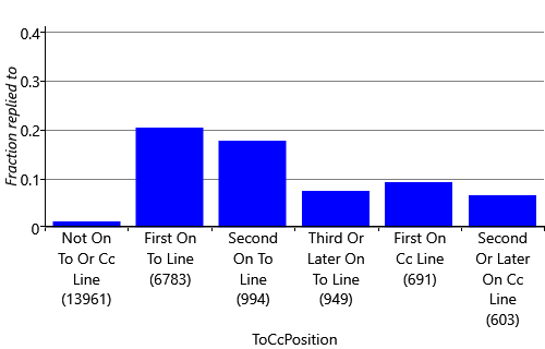
We can improve our feature to capture cues like this by giving it multiple states, one for each of the bars of Figure 4.8. So the states will be: {NotOnToOrCcLine, FirstOnToLine, SecondOnToLine, ThirdOrLaterOnToLine, FirstOnCcLine, SecondOrLaterOnCcLine}. Now we just need to work out what the output of the feature should be, to be suitable for our model (the second criterion). We could try returning a value of 0.0 for NotOnToOrCcLine, 1.0 for FirstOnToLine and so on up to a value of 5.0 for SecondOrLaterOnCcLine. But, according to Assumptions0 4.3 (that the score changes by the weight times the feature value) this would mean that the probability of reply would either steadily increase or steadily decrease as the value changes from 0.0 through to 5.0. Figure 4.8 shows that this is not the case, since the reply fraction goes up and down as we go from left to right. So such an assumption would be incorrect. In general, we want to avoid making assumptions which depend on the ordering of some states that do not have an inherent ordering, like these. Instead we would like to be able to learn how the reply probability is affected separately for each state.
To achieve this we can modify the feature to output multiple feature values, one for each state. We will use a value of 1.0 for the state that applies to a particular email and a value of 0.0 for all other states – this is sometimes called a one-hot encoding. So an email where the user is first on the To line would be represented by the feature values . Similarly an email where the user is first on the Cc line would be represented by the feature values . By doing this, we have effectively created a group of related binary features – however it is much more convenient to think of them as a single ToCcPosition feature which outputs multiple values.

To avoid confusion in terminology, we will refer to the different elements of such a feature as feature buckets – so the ToCcPosition feature contains six feature buckets. For a particular email, you can imagine the one-hot encoding of a feature to be like throwing a ball that lands in one of the buckets.
Using this terminology, the plate across the features in our factor graph should now be interpreted as being across all buckets of all features, so that each bucket has its own featureValue and its own associated weight. This means that the weight can be different for each bucket of our ToCcPosition feature – and so we are no longer assuming that the reply probability steadily increases or decreases across the buckets.
Numeric features
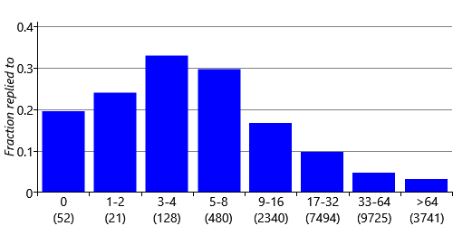
We also need to create features that encode numeric quantities, such as the number of characters in the email body. If we used the number of characters directly as the feature value, we would be assuming that longer emails mean either always higher or always lower reply probability than shorter emails. But in fact we might expect the user to be unlikely to respond to a very short email (“Thanks") or a very long email (such as a newsletter), but may be likely to respond to emails whose length is somewhere in between. Again, we can investigate these beliefs by plotting the fraction of emails replied to for various body lengths. To get a useful plot, it is necessary to group together emails with similar lengths so that we have enough emails to estimate the reply fraction reliably. In Figure 4.9, we label each bar in the bar chart with the corresponding range of body lengths. The range of lengths for each bar is roughly double the size of the previous one, and the final bar is for very long emails (more than 1023 characters).
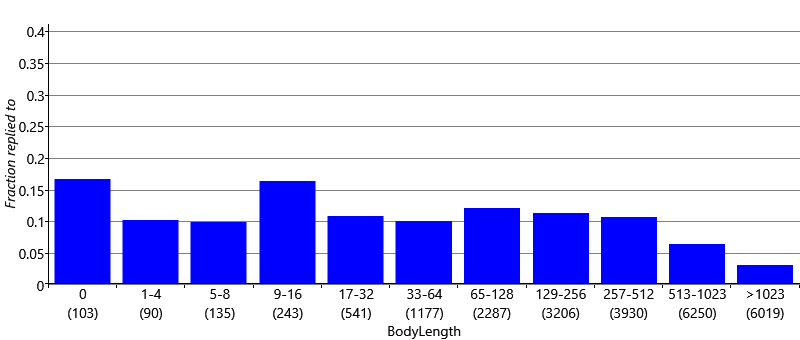
There are several aspects of this plot that are worthy of comment. Zero-length emails have a quite high reply probability, probably because these are emails where the message was in the subject. As we anticipated, very short emails have relatively low reply probability and this increases to a peak in the 9-16 characters and is then roughly constant until we get to very long emails of 513 characters or more where the reply probability starts to tail off. To pick up on these changes in the probability of reply, we can use the same approach as we just used for ToCcPosition and treat each bar of our plot as a different feature bucket. This gives us a BodyLength feature with 11 buckets. Emails whose length fall into a particular length range, such as 33-64 characters, all map to a single bucket. This mapping encodes the assumption that the reply probability does not depend on the exact body length but only on which range that length falls into.
Features with many, many states
We might expect that the sender of an email would be one of the most useful properties for predicting whether a user will reply or not. But why rely on belief, when we can use data? Figure 4.10 shows the fraction of emails replied to for the twenty most frequent senders for User35CB8E5. As you can see there is substantial variation in reply fraction from one sender to another: some senders have no replies at all, whilst others have a high fraction of replies. A similar pattern holds for the other users in our data set. So indeed, the sender is a very useful cue for predicting reply.
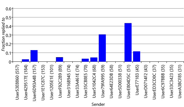
To incorporate the sender information into the feature set, we can use a multi-state Sender feature, with one state for each sender in the data set. For example, User35CB8E5 has 658 unique senders in the training and validation sets combined. This would lead to a feature with 658 buckets of which 657 would have value 0.0 and the bucket corresponding to the actual sender would have value 1.0. Since so many of the feature bucket values would be zero, it is much more efficient to change our factor graph to only include the feature buckets that are actually ‘active’ (non-zero). A suitably modified factor graph is shown in Figure 4.11.
|
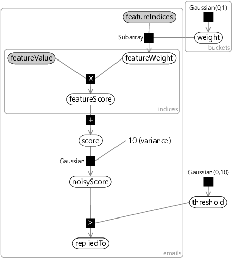
In this modified graph, the feature values for an email are represented by the indices of non-zero values (featureIndices) along with the corresponding values at these indices (featureValues). We use the Subarray factor that we introduced back in section 2.4 to pull out the weights for the active buckets (featureWeight) from the full weights array (weight). This new factor graph allows features like the Sender feature to be added without causing a substantial slow-down in training and classification times. For example, training on User35CB8E5’s training set takes 9.2 seconds using the old factor graph but just 0.43 seconds using this new factor graph. This speed up would be even greater if we had trained on more emails, since there would be more unique senders.
An initial feature set
Now that we know how to encode all the different types of data properties, we can complete our initial feature set, ready to start experimenting with. To encode remaining data properties, we add three further features: FromMe, HasAttachments and SubjectLength whose feature buckets and reply fractions are shown in Figure 4.12.
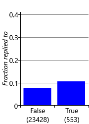
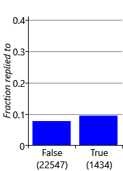
As we discussed back in section 4.1, we removed the content of the subject lines and email bodies from the data set and so cannot add any features to encode the actual words of the subject or of the email body. To build the classifier for the Exchange project, anonymised subject and body words were used from voluntarily provided data. As you might expect, including such subject and body word features did indeed help substantially with predictive accuracy.
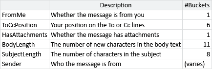
Our initial feature set, with six features, is shown in Table 4.4.
Now that we have a classification model and a feature set, we are ready to see how well they work together to predict whether a user will reply to a new email.
one-hotA way of encoding a 1-of- choice using a vector of size . The vector is zero everywhere except at the position corresponding to the choice, where there is a one. So if there are three options, the first would be encoded by , the second by and the third by .
feature bucketsLabels which identify the values for a feature that returns multiple values. For example, the ToCcPosition feature in Figure 4.8 has six feature buckets: NotOnToOrCcLine, FirstOnToLine, SecondOnToLine, ThirdOrLaterOnToLine, FirstOnCcLine and SecondOrLaterOnCcLine. For this feature the value associated with one of the buckets will be 1.0 and the other values will be 0.0, but for other features multiple buckets may have non-zero values.