8.2 Decision Tree
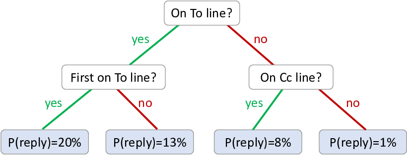
A decision tree is a classifier that makes use of a tree structure to make predictions over a desired target variable. The tree starts at a root node and then contains multiple branching points, where a binary feature is applied at each branching point. Each ‘leaf’ of the tree contains the predictive distribution used for data items that reach that leaf. For example, Figure 8.2 shows a decision tree which predicts whether an email will be replied to – the problem that we explored back in Chapter 4.
To use this decision tree to make a prediction for a particular email, we start by evaluating the top (root) feature for the email. In Figure 8.2, the first feature is: ‘is the user is on the To line for the email?’. If the user is on the To line, we follow the ‘yes’ path to the left, otherwise we follow the ‘no’ path to the right. Suppose we followed the ‘yes’ path – we then get to the feature ‘is the user first on the To line?’. Suppose the user is indeed first on the To line, we again follow the ’yes’ path to the first leaf node. This leaf node contains a probability of reply of , so the tree predicts a probability of replying to this particular email. We will see later how these probabilities, and the structure of the tree itself, can be learned from data.
We’d like to understand the assumptions baked into this prediction process. Unlike for Latent Dirichlet Allocation, there is no standard factor graph for us to analyse. A decision tree is normally described as an algorithm, rather than as a probabilistic model. So our first challenge is to try and represent a decision tree as a probabilistic model, by constructing a factor graph corresponding to the algorithm.
Factor graph for a decision tree
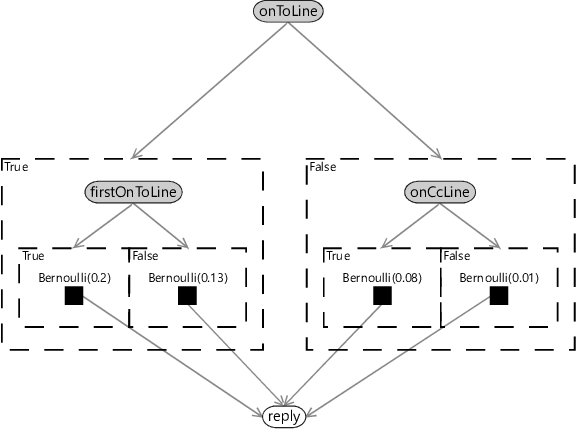
In a decision tree, the root feature controls whether to use the left half of the tree or the right half of the tree. Effectively it switches off the half that is not being used. Similarly, each feature below the root can be thought of as switching off one half of the tree below it. If we switch off half the graph sequentially down from the root, we end up with a single leaf node being left switched on.
Viewing a decision tree this way, we can model its behaviour using gates. The root feature is the selector for a pair of gates, each containing half of the tree. The pair of gates are set up so that one is on when the root feature is true and the other is on when the root feature is false. Within the gate for the left-hand side of the tree, we then repeat this idea. We have a variable for the left-hand feature controlling a pair of gates nested inside the top level gate. Similarly, the gate for the right-hand side of the tree has another pair of gates controlled by the right-hand feature. This construction continues recursively down to the bottom of the tree. When a leaf is reached, we place a factor corresponding to the predictive distribution for that leaf, such as a Bernoulli distribution. All such leaf node factors connect to the single variable which is being predicted.
Applying this construction to the decision tree of Figure 8.2 gives the factor graph of Figure 8.3
In this factor graph, the feature variables are shown as observed (shaded), since the features can be calculated from the email and so are known. The only other variable is the unobserved reply variable that we want to make a prediction for. The nested gates are set up so that only one of the four factor nodes is switched on, depending on the values of the feature variables. This switched-on factor directly provides the predictive distribution for the reply variable.
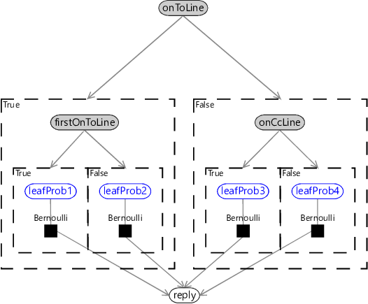
In Figure 8.3, the leaf probabilities are fixed by the four Bernoulli factors. If we want to learn these probabilities, we need to make them into variables, as shown in Figure 8.4.
With the leaf probabilities observed, we can apply a standard inference algorithm to this factor graph to make predictions. Conversely, if the reply variable is observed, we can use the exact same algorithm to learn the leaf probabilities. We could further extend the factor graph to learn which feature to use at each branching point, by adding a gate in a plate that switches between all possible features. Inference of the selector variable for that gate would correspond to learning which feature to apply at that point in the tree. For now though, we will limit ourselves to using the current factor graph to analyse the assumptions that it contains.
What assumptions are being made?
We can use our factor graph to understand the assumptions encoded in a decision tree classifier. It will be informative to compare these assumptions to the ones we made when designing the classifier of Chapter 4. Since both models make use of features of the data, they both make the core assumption that feature values can always be calculated for any data item. But beyond this, the two models make very different assumptions about how feature values combine to give a predictive distribution.
In Chapter 4, the effect of changing the value of one feature was always the same, no matter what the values of other features were (see Table 4.3). This is not true for a decision tree – the leaf node that is reached depends on the value of every feature in the path leading to that leaf. Changing a feature may even do nothing at all, if the feature is not on the path from the root to the currently switched-on leaf. In fact, given that the number of features is usually large compared to the depth of the tree (the number of features from the root to a leaf), changing a randomly selected feature is likely to have no effect! The relevant assumption that the decision tree is making is:
- The predicted probability will only change if one of a small subset of features changes.
To explore this assumption further, consider the set of features we might wish to use for our email prediction problem. Our small initial feature set in Table 4.4 had six features, many of which had multiple buckets. To use these features in a decision tree, they would have to be converted into binary features. For example, if we created one binary feature for each bucket, we would have around 30 binary features. When learning a decision tree, we would need to select one of these features at each branching point. A decision tree with depth five would have branching points, each of which would need to be assigned a feature. However, for any given email, only five features would lie on the path from the root to the selected leaf for that email. Changing any feature apart from those five would have no effect on the predicted probability of reply.
It follows from Assumptions0 8.1 that the decision tree classifier completely ignores any useful information contained in features other than those on the selected path. Whilst we might expect a few features to dominate in making a prediction, that does not mean we would expect other features to contain no useful information whatsoever. The consequence of this assumption is that the decision tree is likely less accurate than it could be, because it is not making use of all the available information.
Now let’s suppose we change the value of a feature that is one of the few affecting the predicted reply probability. How much do we expect the reply probability to change? In Table 4.3 we assumed that a change in a single feature normally has a small effect on the reply probability, sometimes has an intermediate effect and occasionally has a large effect. But for a decision tree, the assumption is again very different. A change in a feature which is on the path to the root will cause a different leaf node to switch on. This node could have a completely different probability of reply. So for a decision tree, the assumption would be:
- Changing a feature value can completely change the predicted probability.
This assumption also has significant consequences. It means that a change in the value of a single feature can totally change the predicted probability. In the context of reply prediction, if the email length is used as a feature, adding a single character to the email could possibly change the leaf node reached. This in turn would change the predicted probability of reply, potentially by a large amount. In practice, we would want the probability to change smoothly as the length of an email changed. This would require a very large decision tree with many leaf nodes, so that we could transition through a series of leaf nodes with slightly different probabilities. In addition, training such a tree would require a great deal of data, in order to accurately learn the reply probability for each of the tree’s many leaves.
So, both of the above assumptions are problematic in terms of making full use of the available data and ensuring that the predicted probability changes appropriately as feature values change. These problems are not just theoretical – decision tree classifiers do indeed suffer from these issues in practice. The solution to both problems is to use more than one decision tree, combined together into a decision forest.
Decision forest

A forest is much better than a single tree.
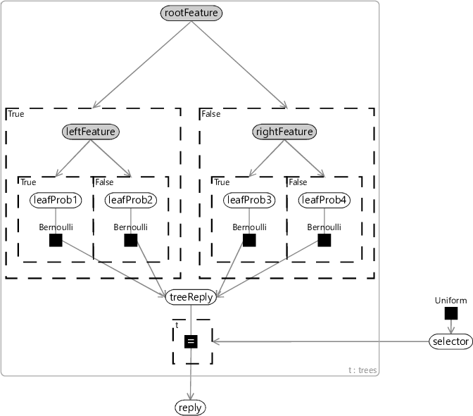
A decision forest is made up of a collection of decision trees, known as an ensemble. Decision forests were first developed by Ho [1995] and then later extended and popularised by Breiman [2001]. Trees in a decision forest are trained so as to be different to one other – for example, by training each tree using different subsets of features or different subsets of the training data. The result of such training is that each tree will give similar, but different, predictive distributions for the same input. To apply the forest, we compute the predictive distribution for each individual tree, and then average them together. A decision forest can also be represented as a factor graph – see Figure 8.5.
A decision forest can overcome both of the issues that arise when using a single decision tree. The first issue, of not making full use of the data, is addressed by including many trees in the forest. Although each tree only makes use of a small subset of features for any data item, these are unlikely to be the same subset from tree to tree. As long as we have sufficient trees, then together they will likely use a large proportion of the available features between them. Overall then the forest will be able to make use of all available information.
Similarly, a change in the value of a single feature is now unlikely to cause a large change in the predictive probability. This is because many of the trees will not have this feature in the switched-on set, and so their predictive probability will remain unchanged. The few trees that do have the feature active could completely change their predictive probabilities, but when we average all probabilities together, the overall change is more likely be small. So, using the decision forest has the effect of smoothing the predictive distribution. However, if there is lots of data to suggest that the probability should change rapidly in response to changing a particular feature, then the trees will end up using the same feature and the probability can change sharply. In practice, use of decision forests improves both accuracy and calibration compared to a single decision tree. The relative simplicity and interpretability of decision forests has led to their use for a wide range of applications. To learn more about using decision forests for a variety of machine learning tasks, take a look at Criminisi et al. [2012].
Review of concepts introduced on this page
decision treeA classifier that uses a tree structure to make predictions for a desired target variable. Each branching point in the tree is associated with a binary feature and each leaf node of the tree is associated with a predictive distribution. To apply the tree, we start at the root and take the left or right path according to the value of the binary feature. This procedure is repeated at each branching point until a leaf node is reached. The output of the classifier is then the predictive distribution at that leaf node.
ensembleA collection of models used together to give better predictive performance than any one of the individual models.
References
[Ho, 1995] Ho, T. K. (1995). Random Decision Forests. Proceedings of the 3rd International Conference on Document
Analysis and Recognition, pages 278–282.
[Breiman, 2001] Breiman, L. (2001). Random Forests. Machine Learning, 45:5–32.
[Criminisi et al., 2012] Criminisi, A., Shotton, J., and Konukoglu, E. (2012). Decision Forests: A Unified Framework for Classification, Regression, Density Estimation, Manifold Learning and Semi-Supervised Learning. Foundations and Trends® in Computer Graphics and Vision, 7(2–3):81–227.