5.5 Modelling star ratings

Our model turns the full range of star ratings into a simple like or dislike, which means it is throwing away a lot of useful information. There is a world of difference between rating a movie at 3 stars and rating it at 5 stars, yet we are treating both of these cases the same. In order to make use of the different star ratings, we need to change our model to work with the full range of ratings rather than a binary like/dislike. Not only will this let us train on star ratings, but we will also be able to predict star ratings – a double benefit!

We can make this change by building on the binary like/dislike model that we have already designed. Inside this model we have an affinity variable which is a continuous number representing how much a person likes a movie. We currently threshold this affinity at zero and say that values above zero mean the person likes the movie and values below zero mean that they do not like the movie. To model different star ratings, we can assume that a higher affinity means that a person will give a higher star rating. More precisely, rather than thresholding only at zero, we can now introduce thresholds for each star rating. If a person’s affinity for a movie is above the threshold for a particular number of stars, then we expect them to give the movie at least that number of stars.

To add these thresholds into our model, we need to make one additional assumption. We need to decide whether the same thresholds should be used for everyone, or whether different people can have different thresholds. Allowing different thresholds might be useful – for example, it is possible that some people give a really bad movie a rating of two stars, while other people give a really bad movie a rating of one star or even half a star. If we want to model these different behaviours, we would need to allow different people to have different thresholds. This can be done but it would introduce problems of data scarcity since some people might not have any ratings for particular thresholds. Rather than tackle these problems, we will make the simplifying assumption that the thresholds are the same for everyone. We can express this assumption precisely, like so:

6. When two people have the same affinity for a movie, they will give it the same number of stars.

Figure 5.19 shows the factor graph for an extended model that encodes this assumption. In this model, we have added a new variable starThreshold which is inside a stars plate, meaning that there is a threshold for each number of stars.

plate of size: traits traits plate of size: people people plate of size: movies movies plate of size: stars stars observed bool variable Whether the person gives the movie at least this number of stars hasStar double[][] variable The person's preference for this trait (their position in trait space). preference double[][] variable The movie's trait value (its position in trait space). trait double[][] variable The affinity threshold for this star rating. starThreshold double[] variable The trait-specific component of the affinity. traitAffinity double variable The affinity that the person has for each movie (more positive means higher probability that they will like the movie). affinity double variable Noisy version of the affinity, to allow for uncertainty in whether a person likes a movie. noisyAffinityGaussian(0,σ²)Gaussian(0,σ²)Gaussian(0,10)×+Gaussian(·,1)>

Figure 5.19Factor graph for a recommender model that can consume and predict star ratings. Ratings are indirectly represented using binary values of the variable hasStar as discussed in the text.

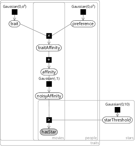
For each movie and person, the observed variable in this graph is now called hasStar. This variable lies inside the stars plate and so has a value for each number of stars. In other words, each single star rating is represented as a set of binary variables. The binary variable for a particular number of stars is true if the rating has at least that number of stars. As an example, a rating of three stars means that the first three binary variables are true and the other two are false. Figure 5.20 shows the relationship between the star rating and the binary values used for the observation of hasStar.

Figure 5.20 Relationship between different star ratings and the binary values used for the hasStar variable in the factor graph of Figure 5.19.

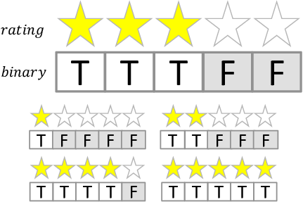
When we train this model, we set hasStar to the observed values given in Figure 5.20 for the corresponding rating. When using the model to make a recommendation, we get back a posterior probability of each binary variable being true. These can be converted into the probability of having a particular number of stars using subtraction. For example, if we predict the probability of having 3 or more stars is 70% and the probability of having 4 or more stars is 60%, then the probability of having exactly 3 stars must be $70\%-60\%=10\%$. Using this trick, we can convert the individual binary probabilities back into separate probabilities for each star rating.

There are a few more details we need to work out before we can train this model. First, in our data set we need to be able to work with half-star ratings, such as $3\frac{1}{2}$ stars. We can handle these by doubling the number of thresholds, so that there are thresholds for both whole and half star ratings. Second, there is a symmetry between the star thresholds and the biases – adding a constant value to all user or movie biases and subtracting that value off all thresholds leads to the same predictions. This can be solved by fixing one of the thresholds to be zero – for our experiments we choose to fix the three star threshold to be zero. Finally, if you look at Figure 5.20, you will note that the first binary value is always true. This means that the affinity must always be greater than the lowest threshold, so we can simply remove it from the model. In our case, that means there will be no threshold for a $\frac{1}{2}$ star and so the lowest threshold will be for $1$ star. With these changes in place, we are now ready to train!

Results with star ratings

Now that we can train on star ratings, we can use the same training data as before (section 5.3) but without converting ratings to like/dislike. When we do this training, we expect that the extra information coming from the star ratings will allow us to locate movies more precisely in trait space. Back in Figure 5.14 we found that, after training on like/dislike, 158 of the movies had a posterior variance of less than 0.2 in each dimension of trait space. After training on star ratings, the number of movies with such low posterior variance increases to 539, showing that we have indeed managed to locate movies more precisely.

As part of training the model, we also learn Gaussian posterior thresholds for each star rating – these are shown in Figure 5.21.

Excel

CSV

Figure 5.21Posterior distributions for star ratings thresholds from 1 star to 5 stars. The threshold for 3 stars is fixed to be exactly zero – all other thresholds have been learned.

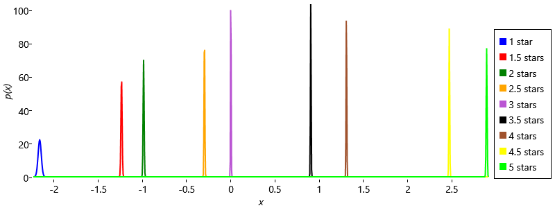
These threshold posteriors are worth looking at. The first thing to note is that the thresholds are ordered correctly from 1 star through to 5 stars, as we would expect. This ordering was not enforced directly in the model since the priors for all the thresholds were the same – instead, the ordering has arisen from the way the model has been trained. Another thing to note is that the posterior distribution for 1 star is much broader than for other thresholds. This is because there are very few half stars and one stars in the training set (to confirm this look back at Figure 5.12). It is these ratings which are used to learn the 1 star threshold and so their relative scarcity leads to higher uncertainty in the threshold location. A final note is that the half star thresholds are generally closer to the star rating above than the one below. For example, the $3\frac{1}{2}$ star threshold is much closer to the 4 star threshold than to the 3 star threshold. This implies that when a person gives $3\frac{1}{2}$ stars to a movie, in their minds they consider that to be almost as good as a 4 star movie, rather than just better than a 3 star movie. Another explanation is that some people may never use half stars (which would explain why they are relatively scarcer than the surrounding whole stars), which would introduce some bias in the inferred thresholds. It is an interesting exercise to think about how the model could be changed to reflect the fact that some people never use half stars.

Using our newly trained model, we can make predictions for exactly the same people and movies as we did in section 5.4. Now our model is predicting star ratings, we can plot the most probable star rating, instead of posterior probabilities of like.

Excel

CSV

(a)Inferred most probable number of stars

 

Excel

CSV

(b)Ground truth number of stars

Figure 5.22Results of our recommender model with star ratings. (a) Predicted most probable ratings, where white squares correspond to five stars, black to half a star and shades of grey represent intermediate numbers of stars. (b) Ground truth ratings using the same colour key.

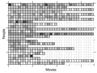
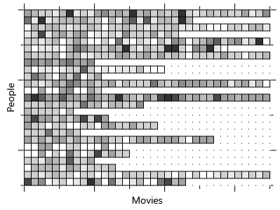
Figure 5.22a shows nicely that we are now able to predict numbers of stars, rather than just like or dislike. Comparing the two plots, we can see that there are sometimes darker or lighter regions in our predictions corresponding to those in the ground truth – but that equally often there are not. It is almost impossible to look at Figure 5.22 and say whether the new model is making better recommendations than the old one. Instead we need to make a quantitative comparison, by re-computing the same metrics as before and comparing the results. For NDCG, we can rank our recommendations by star rating and compute the metric exactly as before. For like/dislike accuracy, we need to convert our star predictions back into binary like/dislike predictions. We can do this by summing up the probabilities of all ratings of 3 stars or higher – if this sum is greater than 0.5, then we predict that the person will like the movie, otherwise that they will dislike it. Figure 5.23 shows that our new model has a significantly improved NDCG than the previous model, demonstrating the value of using the full star ratings. The improvement even shows up in our relatively insensitive fraction-correct metric, although the change is much smaller.

Excel

CSV

(a)Fraction of predictions correct

Excel

CSV

(b)Average NDCG@5

Figure 5.23Comparison of two metrics for the old like/dislike model and the new model with star ratings. The star ratings model gives a significant boost to NDCG, and even shows a small improvement in like/dislike accuracy.

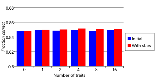
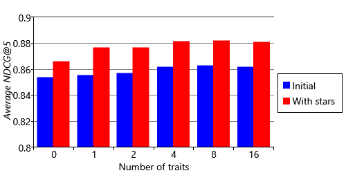
Because we add together probabilities of different star ratings when computing that the like/dislike accuracy metric, we are throwing away information about our recommendations. For example, we are throwing away whether we predicted 3, 4 or 5 stars. The result will be to make the metric less sensitive to improvements in accuracy. We only computed it for Figure 5.23 so that we could compare to the results of the initial model. Now that we have predictions of star ratings, we need to replace this metric with a new one that can make use of ratings. For this new metric, we could look at the fraction of times that the predicted rating correctly matched the ground truth rating. However, this would mean that a prediction that is half a star out would be treated the same as one that is four stars out. Instead, we can look at how far the predicted number of stars was from the actual number of stars, so that the error is:

In equation (5.1), the vertical bars mean that we take the absolute size of the difference. For example, if the prediction is two stars and the ground truth is five stars, the error will be 3.0. The error will also be 3.0 if we swap these over so that the prediction is five stars and the ground truth is two stars. Because we use this absolute size, we call this error the absolute error. To compute a metric over all predictions, we average the absolute errors of each prediction, giving a metric called the mean absolute error (MAE).

Excel

CSV

Figure 5.24Mean absolute error for different numbers of traits in our new star rating model. The MAE generally decreases slightly as we increase the number of traits.

Figure 5.24 shows this metric computed for varying numbers of traits in our new model. Taking all three metrics together, having more traits generally seems to give better quality recommendations. So we can choose to use the 16-trait version of our latest model which gives an NDCG@5 of 0.881 and an MAE of 0.663. While this gives us our best performing recommender system yet, it would still be good to make further improvements. In the next section we’ll diagnose where we are still making mistakes and look at one way to further improve our recommendation accuracy.