5.6 Another cold start problem

When we plotted the position of movies in trait space (Figure 5.14), we showed only those movies where the position was known reasonably accurately (that is, where the posterior variance was low). It follows that there are many movies where the posterior variance is larger, possibly much larger. This means that we essentially do not know where some movies are in trait space. We might expect these to be the movies which do not have many ratings. If we do not know where some movies are in trait space, then we might expect the accuracy of recommendations relating to such movies to be low. How can we diagnose if this is the case?

First, it would be useful to understand how many ratings each movie typically has. Figure 5.25 shows the number of ratings for each movie in the data set as a whole, with the movies ordered from most ratings on the left to least ratings on the right.

Excel

CSV

Figure 5.25The number of ratings given for each movie in the data set as a whole. The movies are ordered from most ratings on the left to least ratings on the right.

From Figure 5.25, we can see that only about 500 of the 9000 movies have more than 50 ratings. Looking more closely, only around 2000 movies have more than 10 ratings. This leaves us with 7000 movies that have 10 or fewer ratings – of which about 3000 have only a single rating! It would not be surprising if such movies cannot be placed accurately in trait space, using rating information alone. As a result, we might expect that our prediction accuracy would be lower for those movies with few ratings than for those with many.

To confirm this hypothesis, we can plot the mean absolute error across the movies divided into groups according to the number of ratings they have in the training set. This plot is shown in Figure 5.26 for an experiment with 16 traits. For this experiment, we added into the validation set the movies that do not have any ratings in the training set (the left-hand bar in Figure 5.26). This provides a useful reference since it shows what the MAE is for movies with no ratings at all. The plot shows that when we have just one rating (second bar), we do not actually reduce the MAE much compared to having zero ratings (first bar). For movies with more and more ratings, the mean absolute error drops significantly, as shown by the third and fourth bars in Figure 5.26. Overall, this figure shows clearly that we are doing better at predicting ratings for movies that have more ratings – and very badly for those movies with just one.

Excel

CSV

Figure 5.26Mean absolute error for movies with different numbers of ratings in the training set, for a model with 16 traits. Each bar is labelled with the range of ratings and, in brackets, the number of movies that fall into that range. For example, the left-hand bar gives the MAE for movies with no ratings in the training set, of which there are 1,015. Comparing the four bars shows that movies with many ratings have substantially lower prediction errors than those with few or zero ratings.

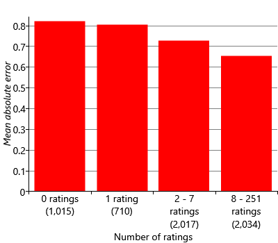
Figure 5.26 confirms that we have an accuracy problem for movies with few ratings. This is particularly troubling in practice since newly released movies are likely to have relatively few ratings but are also likely to be the most useful recommendations for users. So how can we solve this problem? Recalling section 4.6 from the previous chapter, we can think of this as another cold start problem. We need to be able to make recommendations about a movie even though we have few or even zero ratings for that movie.

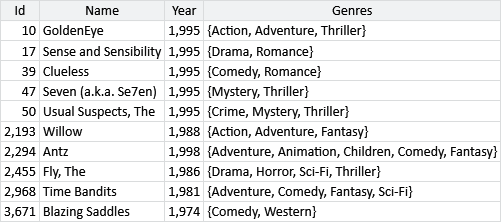
Apart from ratings, what other information do we have that could be used to improve our recommendations? Looking at our data set, we see that it also includes the year of release and the genres that each movie belongs to. A sample of this additional information is shown in Table 5.4.

Excel

CSV

Table 5.4A sample of the additional information available for each movie.

If we could use this information to place our movies more accurately in trait space, perhaps that would improve our recommendations for movies where we only have a few ratings. We can try this out by adding this information to our model using features, just like we did in the previous chapter.

Adding features to our model

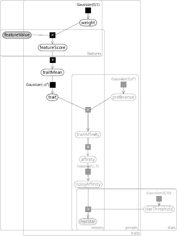
To add features to our recommender model, we can re-use a chunk of the classification model from section 4.3. Specifically, we will introduce variables for the featureValue for each movie and feature, along with a weight for each feature and trait. As before, the product of these will give a featureScore. The sum of these feature scores will now be used as the mean for the trait prior – which we shall call traitMean. It follows that the prior position of the movie in trait space can now change, depending on the feature values, before any ratings have been seen! The resulting factor graph is shown in Figure 5.27 – the unchanged part of the graph has been faded out to make the newly-added part stand out.

plate of size: traits traits plate of size: people people plate of size: features features plate of size: movies movies plate of size: stars stars observed bool variable Whether the person gives the movie at least this number of stars hasStar observed double[][] variable The value of this feature for this movie. featureValue double[][] variable The weight for this feature for this trait. weight double[][] variable The person's preference for this trait (their position in trait space). preference double[][] variable The movie's trait value (its position in trait space). trait double[][] variable The affinity threshold for this star rating. starThreshold double[] variable The contribution of this feature to the trait mean for this movie. featureScore double variable The mean of the prior distribution for this movie, given its feature values. traitMean double[] variable The trait-specific component of the affinity. traitAffinity double variable The affinity that the person has for each movie (more positive means higher probability that they will like the movie). affinity double variable Noisy version of the affinity, to allow for uncertainty in whether a person likes a movie. noisyAffinityGaussian(0,σ²)Gaussian(0,1)×+Gaussian(·,σ²)Gaussian(0,10)×+Gaussian(·,1)>

Figure 5.27Factor graph for a recommender model that can consume feature values for individual movies. To emphasize the variables and factors which have been added, the remaining parts of the graph have been faded out.

In taking this chunk of model from the previous chapter, we must remember that we have also inherited the corresponding assumptions. Translated into the language of our model, these are:

7. The feature values can always be calculated, for any movie.
8. If a movie’s feature value changes by $x$, then each trait mean will move by $\mathit{weight}\times x$ for some fixed, continuous, trait-specific weight.
9. The weight for a feature and trait is equally likely to be positive or negative.
10. A single feature normally has a small effect on a trait mean, sometimes has an intermediate effect and occasionally has a large effect.
11. A particular change in one feature’s value will cause the same change in each trait mean, no matter what the values of the other features are.

We explored these assumptions extensively in the previous chapter, so will not discuss them again here. However, it would be a worthwhile exercise to spend some time reflecting on how each assumption will affect the behaviour of our recommender system.

As in the previous chapter, we need to decide how to represent our movie information as features. The features that we will use are:

1. A constant feature set to 1.0 for all movies, used to capture any fixed bias.
2. A ReleaseYear feature which is represented using buckets, much like the BodyLength feature we designed in section 4.4. We choose the buckets to be every ten years until 1980 and then every five years after that – giving 17 buckets in total.
3. A Genres features which has the same design as the Recipients feature from section 4.5. That is, a total feature value of 1.0 is split evenly among the genres that a movie has. So if a movie is a Drama and a Romance, the Drama bucket will have a value of 0.5 and the Romance bucket will also have a value of 0.5.

This data set contains additional information about the movies but not about the people giving the ratings (such as age or gender). If we had such additional information we could incorporate it into our model using features, just as we did for movies. All we would need to do is add a features model for the mean of the preference prior of the same form as the one used for the trait prior in Figure 5.27. The resulting model would then be symmetrical between the movies/traits and people/preferences.

Results with features

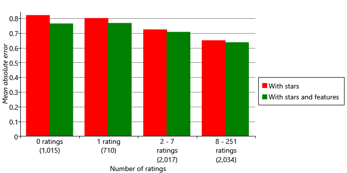
Let’s see what effect using movie features has on our accuracy metrics. Figure 5.28 shows the mean absolute error for models with and without features, for groups of movies with different numbers of ratings. We can see that adding features has improved accuracy for all four groups, with the biggest improvements in the groups with zero ratings. While there is still better accuracy for movies with more ratings, using features has helped narrow the gap between these movies and movies where few ratings are available.

Excel

CSV

Figure 5.28Including feature information in our model has reduced the prediction error, particularly for movies with only no ratings in the training set.

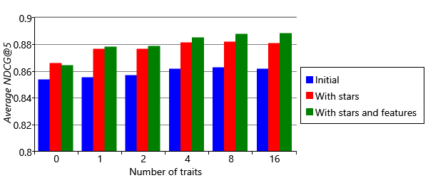
We can also look at the effect of using features on our overall metrics. These are shown for different numbers of traits in Figure 5.29. For comparison with previous results, we once again exclude ratings for movies that do not occur in the training set (that is, the left-hand bar of Figure 5.28). The chart shows that features increase accuracy whichever metric we look at. Interestingly, this increase is greater when more traits are used. The explanation for this effect is that we are not directly using features to make recommendations but instead we are using them indirectly to position movies in trait space. Using more traits helps us to capture the feature information more precisely, since a position in trait space conveys more information when there are more traits.

Excel

CSV

(a)Mean absolute error (MAE)

  

Excel

CSV

(b)Average NDCG@5      

Figure 5.29Comparison of MAE and NDCG metrics for each of our models. Note that MAE cannot be calculated for the initial model because it does not predict star ratings. According to these metrics, feature increases accuracy for any model with at least one trait, with the increase being larger as more traits are used.

Overall, using features has provided a good increase in accuracy, particularly for items with few ratings. This means that our model should now do a much better job of making recommendations for new movies – which is a very desirable characteristic!

Final thoughts

In this chapter, we have developed a recommender model that can consume either like/dislike labels or full star ratings. The model can also make use of additional information about the items being recommended. As a result, this model is already enough to be valuable for many customers of Azure machine learning – and indeed is very close to the one that was actually used in Azure ML. The main difference is that the Azure ML model can also learn personalised star ratings thresholds. This was achieved by moving the starThreshold variable inside the people plate and giving each threshold a suitably informative prior, to allow for data scarcity.

In developing our model, we have assumed that a good recommendation is one where the user will rate the item highly, but in fact this may not be the case. A science fiction fan may rate Star Wars highly, but it would be a poor recommendation since they would almost certainly already seen it. In other words, a good recommendation is for a movie that you are likely to enjoy but not to have already seen. Real recommendation systems keep a record of what movies a person has seen through the system and these are automatically removed from any list of recommendations. But such systems have no knowledge of what movies have been watched outside of the system. We could modify our model to predict both whether someone would like a movie and whether they are likely to have seen it. Using both of these predictions together would lead to more valuable recommendations.

Similar items are nearby in trait space.

By learning the positions of items in trait space, we have also learned which items are similar, since these will be close to each other. Given a target item, we can find similar items by searching for nearby items in trait space. More precisely, we can do this by making recommendations for an imaginary person located at the same position in trait space as the target item. The result of this process is useful for making item-specific recommendations, such as “people who liked this movie, also liked”. Item relatedness can also be used to improve the diversity in a set of recommendations. For example, we might not want to have two very similar movies in a list of recommendations (such as two movies in the same series). We could use the distance between the movies in trait space to remove such similar movies and so create a more diverse list of recommendations.

There are further model extensions that could usefully be made. One would be to make use of implicit feedback about an item. For example, many people never rate any movie, but instead just watch them. Even in this case, there is still useful information about the movies that the person likes. We may assume that they watch movies that they expect to like – so watching a movie is an implicit signal that the person liked the movie. It is harder to get an implicit signal that a person did not like a movie and so often implicit feedback provides positive-only data. In other words we have only the good ratings and none of the bad ones. Having a model that can cope with such positive-only data would be very useful – the most common approach today is to treat a random sample of unrated movies as if they were negatively rated.

Even when we do have ratings, the information about which ratings we have and which we do not have is very valuable. Having a rating is a bit like watching a movie – it provides a positive signal about liking the movie. The best performing recommender systems make use of missing ratings to provide information about what a person likes or dislikes. With any piece of data that can be missing, we can model whether or not it is missing, as well as modelling the data itself. In the next chapter, we will discuss different kinds of missing data and how to handle them – in the very different scenario of understanding childhood asthma.