5.2 Multiple traits and multiple people

Our model with just one trait is not going to allow us to characterize movies very well. To see this, take another look at Figure 5.4:

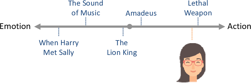
Using just the action/emotion trait, we can hardly distinguish between The Lion King and Amadeus since these have very similar positions on this trait line. So for the woman in this figure, we would not be able to recommend films like Amadeus (which she likes) without also recommending films like The Lion King (which she doesn’t like).

We can address this problem by using additional traits. If we include a second trait representing how escapist or realist the film is, then each movie will now have a position on this second trait line as well as on the original trait line. This second trait value allows us to distinguish between these two movies. To see this, we can show the movies on a two-dimensional plot where the escapist/realist trait position is on the vertical axis, as shown in Figure 5.8.

Figure 5.8Two-dimensional plot where the new vertical axis shows how escapist or realist a movie is. Dotted lines show that the horizontal position of the movies has not changed.

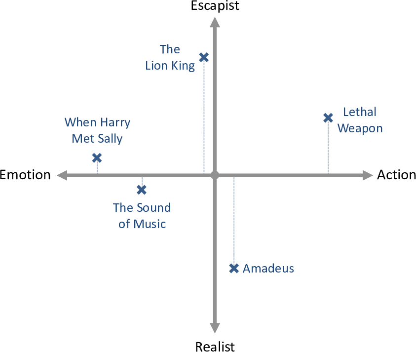
In Figure 5.8, the more escapist movies have moved above the emotion/action line and the more realist movies have moved below. The left/right position of these movies has not changed from before (as shown by the dotted lines). This two-dimensional space allows Amadeus to be move far away from the The Lion King which means that the two movies can now be distinguished from each other.

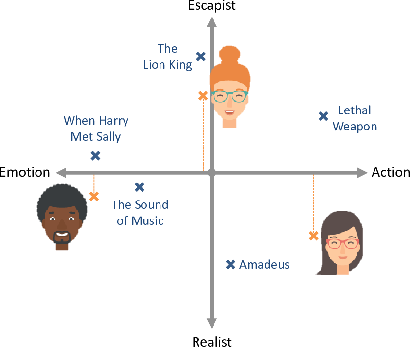
Given this two dimensional plot, we can indicate each person’s preference for more escapist or realist movies by positioning them appropriately above or below the emotion/action line, as shown in Figure 5.9. Looking at this figure, you can see that the woman from Figure 5.4 has now moved below the emotion/action line, since she has a preference for more realistic movies. Her preference point is now much closer to Amadeus than to The Lion King – which means it is now possible for our system to recommend Amadeus without also recommending The Lion King.

Figure 5.9Placing people on the two-dimension plot allows us to capture their preferences for escapist/realist movies, whilst still representing their preferences for emotional/action movies.

We have now placed movies and people in a two-dimensional space, which we will call trait space. If we have three traits then trait space will be 3-dimensional, and so on for higher numbers of traits. We can use the concept of trait space to update our first two assumptions to allow for multiple traits:

1. Each movie can be characterized by its position on the trait line in trait space, represented as a continuous number for each trait.
2. A person’s preferences can be characterized by a position on the trait line in trait space, again represented as a continuous number for each trait.

Assumptions0 5.3 does not need to be changed since we are combining each trait and preference exactly as we did when there was just one trait. However, we do need to make an additional assumption about how a person’s preferences for different traits combine together to make an overall affinity.

4. The effect of one trait value on whether a person likes or dislikes a movie is the same, no matter what other trait values that movie has.

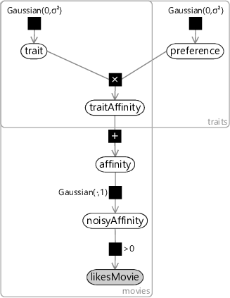
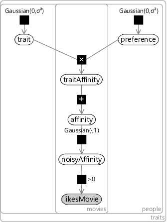
We can encode this assumption in our model by computing a separate affinity for each trait (which we will call the traitAffinity) and then just add them together to give an overall affinity. Figure 5.10 gives the factor graph for this model with a new plate over traits that contains the trait value for each movie, the preference for each person and the traitAffinity, indicating that all of these variables are duplicated per trait.

plate of size: traits traits plate of size: movies movies observed bool variable Whether the person likes the movie. likesMovie double[] variable The person's preference for this trait (their position in trait space). preference double[][] variable The movie's trait value (its position in trait space). trait double[] variable The trait-specific component of the affinity. traitAffinity double variable The affinity that the person has for each movie (more positive means higher probability that they will like the movie). affinity double variable Noisy version of the affinity, to allow for uncertainty in whether a person likes a movie. noisyAffinityGaussian(0,σ²) Gaussian(0,σ²)×+Gaussian(·,1)>0

Figure 5.10Factor graph for combining together multiple traits.

This model combines together traits in exactly the same way that we combined together features in the previous chapter. Once again, it leads to a very similar factor graph – to see this, compare Figure 5.10 to Figure 4.5. The main difference again is that we now have an unobserved trait variable where before we had an observed featureValue. This may seem like a small difference, but the implications of having this variable unobserved are huge. Rather than using features which are hand-designed and provide given values for each item, we are now asking our model to learn the traits and the trait values for itself! Think about this for a moment – we are effectively asking our system to create its own feature set and assign values for those features to each movie – all by just using movie ratings. The fact that this is even possible may seem like magic – but it arises from having a clearly defined model combined with a powerful inference algorithm.

One new complexity arises in this model around the choice of the prior variance $\sigma^2$ for the trait and preference variables. Because we are now adding together several trait affinities, we risk changing the range of values that the affinity can take as we vary the number of traits. To keep this range approximately fixed, we set $\sigma^2 = 1/\sqrt{T}$ where $T$ is the number of traits. The intuition behind this choice of variance is that we would then expect the trait affinity to have a variance of approximately $1/\sqrt{T}\times 1/\sqrt{T}= 1/T$. The sum of $T$ of these would have variance of approximately $1$, which is the same as the single trait model.

Learning from many people at once

If we try to use this model to infer traits and preferences given data for just one person, we will only be able to learn about movies which that person has rated – probably not very many. We can do much better if we pool together the data from many people, since this is likely to give a lot of data for popular movies and at least a little data for the vast majority of movies. This approach is called collaborative filtering – a term coined by the developers of Tapestry, the first ever recommender system. In Tapestry, collaborative filtering was proposed for handling email documents, where “people collaborate to help one another perform filtering by recording their reactions to documents they read” [Goldberg et al., 1992]. In our application we want to filter movies by recording the ratings (that is, reactions) that other people have to the movies they watch – a different application, but the underlying principle is the same.

To extend our factor graph to handle multiple people, we add a new plate over people and put all variables inside it except the trait variable, (which is shared across people). The resulting factor graph is shown in Figure 5.11. Looking at this factor graph, you can see that it is symmetric between people and movies. In other words, we could swap over people and movies and we would end up with exactly the same model!

plate of size: traits traits plate of size: people people plate of size: movies movies observed bool variable Whether the person likes the movie. likesMovie double[][] variable The person's preference for this trait (their position in trait space). preference double[][] variable The movie's trait value (its position in trait space). trait double[] variable The trait-specific component of the affinity. traitAffinity double variable The affinity that the person has for each movie (more positive means higher probability that they will like the movie). affinity double variable Noisy version of the affinity, to allow for uncertainty in whether a person likes a movie. noisyAffinityGaussian(0,σ²) Gaussian(0,σ²)×+Gaussian(·,1)>0

Figure 5.11Factor graph for a recommender model which can learn from like/dislike data pooled across many people.

In this model we have chosen to threshold the noisyAffinity at zero, roughly corresponding to the assumption that half the ratings will be ‘like’ and half will be ‘dislike’. This is quite a strong assumption to be making, so we could instead learn this threshold value as we did for the classifier model. Instead we will do something better – we will make a change that effectively allows different thresholds to be learned for each movie and for each person. We will add a bias variable per movie and a bias variable per user and include these two variables in the sum when we compute the total affinity. Introducing biases in this way allows the model to capture the general popularity of a movie and the degree to which each person likes movies in general. For example, if a user likes nearly every movie then they will get a high user bias. Similarly, if a movie is liked by nearly every user then it will get a high movie bias.

We can add in biases without changing the factor graph from the one in Figure 5.11 – all we do is use a traits plate that is two bigger than the desired number of traits and fix the first preference value and the second trait value to be exactly 1.0. Then, the first trait value will be the bias for a movie and the second preference value will be the bias for a person. We will use this trick to include biases in all models in this chapter, but they will not be shown explicitly in the factor graphs, to keep them uncluttered.

Our final assumption is that we do not need any more variables in our model – or to put it another way:

5. Whether a person will like or dislike a movie depends only on their preferences for the movie’s traits and not on anything else.

We will assess the validity of this assumption shortly, but first let’s put all of our assumptions together in one place so that we can review them all (Table 5.2).

Assumptions0 5.1 seems reasonable since we can theoretically make trait space as large as we like, in order to completely characterize any movie – for smaller numbers of traits this assumption will hold less well, but still hopefully be a good enough assumption for practical purposes. Assumptions0 5.2 assumes that a person’s tastes can be well represented by a single point in trait space. Quite possibly, people could occupy multiple points in trait space, for example a person may like both children’s cartoons and very violent movies, but nothing in between. However, it may be reasonable to assume that such people are rare and so a person occupying a single point is a decent assumption in most cases.

Assumptions0 5.3 and Assumptions0 5.4 relate to how movie and person traits combine together to give an affinity. Perhaps the most questionable assumption here is Assumptions0 5.4 which says that the effect of each trait does not depend on the other traits. In practice, we might expect some traits to override others or to combine in unusual ways. For example, if someone only likes action movies that star Arnold Schwarzenegger, but dislikes all the other kinds of movies that he appears in – then this would be poorly modelled by these assumptions because the ‘stars Arnold Schwarzenegger’ trait would have a positive effect in some cases and a negative effect in others.

A person may only like some movies at particular times of year

Finally, we have Assumptions0 5.5 which says that whether someone likes or dislikes a movie will depend only on their preferences for the movie’s traits – in fact it may depend on many other things. For example, the time of year may be a factor – someone may love Christmas movies in December but loathe them in January. Another factor could be the other people that are watching the movie – whether someone enjoys a movie could well depend on who is watching it with them. Following this line of thought, we could imagine a recommendation system that recommends movies for groups of people – this has in fact been explored by, for example, Zhang et al. [2015]. Other things that could influence a person’s enjoyment could include: the time of day or time of week, their emotional state (do they want a happy movie or a sad one? do they want to be distracted from real life or challenged?) and so on. In short, there is plenty to question about Assumptions0 5.5 – but it’s fine to stick with it for now and then consider extending the model to capture additional cues later on.

So let’s keep the model as it is and use it to make some recommendations!